Kallen A. Understanding Biostatistics

Подождите немного. Документ загружается.

ANALYSIS DONE THE VERTICAL WAY 221

above refers to the median of the differences ln X − ln Y = ln X/Y , and by exponentiation

we ﬁnd that the drug effect is estimated as 14% with 95% conﬁdence interval (4.3, 48)% for

active versus placebo.

The reader may have noted that the conﬁdence interval for the Hodges–Lehmann estimate

in Figure 8.4 does not quite ﬁt with the pointwise conﬁdence interval curves. That is because

the conﬁdence interval for the Hodges–Lehmann estimate in this case was obtained in the

way it is usually computed and not the correct way. To understand the difference we need to

take a closer look at how the pointwise conﬁdence intervals for H(z) are constructed.

We ﬁrst take z = 0 and focus on the Wilcoxon probability. The basic fact that underlies the

computation of the conﬁdence interval for P

is the observation that the stochastic variable



∞

−∞

(x)dF

(x) has an asymptotic Gaussian distribution with mean P

and with

the variance σ

), with the function σ

(P) deﬁned by

nm σ

(P) =(m − 1)





∞

−∞

G(x)

dF (x) − P



+ (n − 1)





∞

−∞

F (x)

dG(x) −(1 − P )



+ P(1 −P).

(8.8)

One derivation of this formula is given in Appendix 8.A, in which the Wilcoxon probability

parameter is discussed as a U-statistic, and where it is also shown that the distribution

of the estimator is asymptotically Gaussian. From this we derive the (approximate)

conﬁdence function

C(P

) = 



− H

σ(P

)



which we can use to obtain knowledge about P

. To get the corresponding expression for

H(z) we only replace G(x)byG(x + z) and P

by H(z) in the integrals above. Denote the

corresponding standard deviation by σ(H(z),z).

In order to get the conﬁdence limits for the Hodges–Lehmann estimate θ, note that for θ

to be the median means that it solves the equation H(θ) = 1/2, which in turn implies that we

obtain knowledge about θ from the conﬁdence function

C(θ) = 



1/2 −H

(θ)

σ(1/2,θ)



This is the correct way to compute the conﬁdence limits for the Hodges–Lehmann estimate.

The standard way, referred to above, is to use the approximation obtained by taking θ = 0

and G(x) = F(x) when we compute the variance. Some calculations shows that the variance

(1/2, 0) equals (n + m + 1)/(12nm), so the conﬁdence limits for θ derived from this would

be the solutions to the equations

(θ) =

± z

α/2



n + m + 1

12nm

There is one further geometric interpretation of P

, shown in Figure 8.5. The dashed

curve in this graph is the path of CDF pairs (F (x),G(x)) inside the unit square, obtained by

varying x. In this graph the value of the Wilcoxon probability parameter P

is the area above

this curve. We can assess the difference between the two distributions from how much this

222 HOW TO COMPARE THE OUTCOME IN TWO GROUPS

0.1

0.2

0.3

0.4

0.5

0.6

0.7

0.8

0.9

G(x)

0.20 0.4 0.6 0.8 1

F(x)

Figure 8.5 The geometric interpretation of the Wilcoxon parameter as an area. P

is the

area above the dashed line, which is estimated by the area above the polygon.

curve departs from the equality line, and a summary measure of this is to see how much P

deviates from 1/2. Another way to state this is as follows. The function K(x) = F (G

−1

(x)) is

a distribution function on (0, 1), and P

is the mean of this function. If F (x) = G(x)wehave

K(x) = x as the uniform distribution on (0, 1), which has mean 1/2. We encountered this type

of curve in the form of ROC curves in connection with diagnostic tests.

The parameter estimation version of the Wilcoxon test (equation (8.6)) is more general

than the shift model and can be applied to all kinds of one-parameter models for the two

distributions. If we assume the AFT model G(x) = F(x/θ) instead, we have that θ should

solve the equation



∞

−∞

G(θx)dF (x) =

A short calculation shows that this means that θ is the median of the distribution for the

variable Z = Y/X, with X and Y as before. For the proportional odds model in equation (8.3)

the corresponding equation for θ is



∞

−∞

θG(x)dF (x)

θG(x) +G

(x)

In either model, we replace CDFs with e-CDFs in order to obtain an estimating equation for

θ from data.

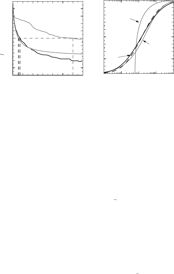
Example 8.1 Figure 8.6 illustrates the different models discussed above, applied to the

sputum data, except that the translation model is written as G(x) = F (x + θ) and the AFT

model is written as G(x) = F (θx), in order to make θ positive in the ﬁrst case and greater

than one in the second. Figure 8.6(a) shows the integrals



∞

−∞

(x, θ)dF

(x) as functions of

θ. The different estimates of θ are obtained from where these curves intersect the horizontal

line at level 1/2. For the shift model we ﬁnd the same estimate as before, the Hodges–

Lehmann estimate. For the AFT model we ﬁnd the estimate 7.18, which is the same estimate

ANALYSIS DONE THE VERTICAL WAY 223

0.1

0.2

0.3

0.4

0.5

0.6

0.7

0.8

0.9

(a) (b)

∞

−∞

(x, θ)dF

(x )

706050403020100

Parameter value θ

0.1

0.2

0.3

0.4

0.5

0.6

0.7

0.8

0.9

Derived F (x )

Sputum count x

Shift model

Proportional

Odds model

AFT

model

Figure 8.6 Fitting different models to the sputum count data, based on the Wilcoxon test. In

(a) the integrals involved are plotted as functions of θ to illustrate how we obtain the estimate;

in (b) the predicted F (x) from the models is compared to the original (dashed curve).

as previously obtained for the Hodges–Lehmann estimate on logged sputum data. Finally, we

ﬁnd the estimate 5.64 for the proportional odds model.

Using these estimates of θ, we can reconstruct F (x) from G(x) for each of the models

and compare them to the original F(x) (which is the dashed curve in the graph). The result is

shown in Figure 8.6(b). We see, as expected, that the pure shift model is poor, but it is hard to

separate the other two models from the original. What really should drive the choice of model

is an understanding of what one wishes to describe.

In order to obtain knowledge about the model parameters we repeat steps we have already

outlined. The general estimating equation is

U(θ) =



∞

−∞

(x, θ)dF

(x) −

= 0,

and we appeal to the CLT to argue that

U(θ) ∈ AsN(0,V

(U(θ))).

It only remains to determine the variance. But this is given by equation (8.8): all we need

to do is put P = 1/2 and replace G(x) with G(x, θ). We therefore ﬁnd that V

(U(θ)) is

1/nm times

(m − 1)



∞

−∞

G(x, θ)

dF (x) + (n − 1)



∞

−∞

F (x)

dG(x, θ) −

(m + n − 3),

224 HOW TO COMPARE THE OUTCOME IN TWO GROUPS

which we estimate by inserting e-CDFs instead of CDFs. The conﬁdence function for θ is

then deﬁned by

C(θ) = 



U(θ)



(U(θ))



We conclude this section by observing that the Wilcoxon test is only a role model for

non-parametric tests, albeit the most important example of such tests. We can deﬁne other

related two-group tests from almost any function a(u) deﬁned on the interval [0, 1] by using

the relation



∞

−∞

a(G(x))dF (x) =



a(u)du,

which is valid for continuous distributions when G(x) = F (x) (we need the integral on the

right to be ﬁnite). If we insert (x) instead of G(x) in the argument for a(u), this provides

us with the framework for many classical linear rank tests. However, using G(x) instead

has its own merits, because it is then clear how to compute the variance and how to do

parameter estimation.

8.5 Some ways to compute p-values

From the discussion so far we can deduce how to compute the p-values for tests of the null

hypothesis F (x) = G(x). However, there are some enhancements of this that justify a separate

discussion on this particular problem.

We start with the t-test. Under the assumption of Gaussian distributions with a common

variance we can compute an exact p-value for the null hypothesis of equal means. This is

because the test statistic (¯y − ¯x)/s

√

−1

+ m

−1

follows a t distribution, based on which we

compute the p-value. In real life the assumptions are never exactly fulﬁlled and the value of

the test statistic is therefore only approximately t-distributed. As a consequence, the p-value

we compute is only an approximation of the ‘true’ p-value. How far off it is in a particular

situation is impossible to assess accurately, since we do not know the exact distribution of the

test statistic. However, we can often argue that the approximation is ﬁt for purpose, because

of the mathematical result described by the CLT. How good the approximation is depends on

the sample size and on how symmetric the data distribution is – in other words, how Gaussian-

like it is. It is the data that are analyzed that matter; sometimes this variable is the change in

an outcome measurement, where both the before and after values may have highly skewed

distributions, while the change is a reasonably symmetric variable.

This discussion on the t-test does not apply to the Wilcoxon test. Here the situation is

different because only a ﬁnite number of values are possible for the test statistic, the rank

sum, given the sample size. Theoretically we can therefore enumerate all the cases, and label

those that lead to a sufﬁciently extreme value for the test statistic. The p-value becomes a

simple fraction. This would be an exact p-value for the null hypothesis, valid whatever the

distribution F(x) looks like, and is the reason why they are called non-parametric tests. The

problem is that unless sample sizes are relatively small, the numbers involved are huge and

time-consuming to compute. As an example, for the sputum data we compute the Wilcoxon

rank sum as 523. To compute the p-value, we look at all possible ways of allocating the

SOME WAYS TO COMPUTE p-VALUES 225

observed data points to the two groups with the group sizes kept constant. For each such

permutation of data we compute the test statistic, and from that we can compute the CDF

for the rank sums. By picking out tails, we can compute the p-value. This is however not a

convenient method in our two-group case, with 40 data points equally divided between two

groups, because there are





≈ 1.4 · 10

such permutations. Because of the sheer size of

this, we do not compute this p-value here, but there are algorithms developed that also allow

us to compute the exact p-values for moderately large data sets.

Unless the sample sizes are small, the CLT provides us with a method to compute approx-

imations to the p-value for the Wilcoxon test, which has been described above. To apply it, we

need to compute the expected rank sum and its variance under the assumption of G(x) = F (x),

which is a pure combinatorial problem, the result of which was given in Box 8.3. Note that

the accuracy depends only on sample sizes, and not on the actual distribution F (x), as was

the case for the t-test.

There is a version of the exact computation that can be applied to the t-test as well, which

we describe in the next example.

Example 8.2 For the t-test, the distribution of the test statistic was deduced from mathemat-

ical operations based on distributional assumptions. An alternative approach is to deduce the

distribution of the test statistic by estimating the combined CDF (x) with its e-CDF 

(x),

and enumerate all possible assignments of groups to this data. For each such assignment we

have one value of the test statistic, and consequently the process gives us the CDF for the test

statistic under these conditions, from which a p-value can be computed as a simple fraction.

A test of the kind described in Example 8.2 is called a randomization test (or permutation

test). The p-values obtained from such tests are often referred to as exact, which they are

if the (combined) sample obtained is the only possible sample. In other words, the p-value

obtained in this way is from a conditional test, where we take the values of the observations

in that particular experiment as given. As an unconditional test, however, it is not exact – how

accurate the p-value is depends on how well the e-CDF of the combined sample approximates

the true CDF. If we apply this procedure to the Wilcoxon rank sum statistic, we derive the

combinatorial p-value described above, since it is the same procedure as was described for the

computation of the exact p-value for the Wilcoxon test. This also implies that its computational

hurdles apply to the randomization tests as well.

A related method, which is also feasible for large samples, is to use bootstrapping. This

method was described in Section 6.7 as a method to estimate the CDF for the test statistic by

repeated resampling. With this method we perform resampling a large number of times and for

each of these samples we compute the test statistic. This gives us an estimate of the distribution

of the test statistic for the actual data, which puts us in a position to compute the appropriate

p-value. This method will be approximate both for the t-test and for the Wilcoxon test. How

good the approximation is depends on how well the two e-CDFs describe their respective

CDFs, and also on how many samples we take.

Example 8.3 For the sputum data we computed the Wilcoxon test statistic as 523. The

two-sided p-value 2(1 − F (523)) can then be computed from a bootstrap-derived estimate of

the distribution F (x) of the rank test based on 10 000 samples, as 0.0021, but it varies slightly

between different runs since tail probabilities need many resamplings. In this case the CDF

226 HOW TO COMPARE THE OUTCOME IN TWO GROUPS

we obtain by bootstrapping is for all practical purposes identical to the Gaussian CDF whose

mean is the expected value of the Wilcoxon ranks statistic, here 410, and whose standard

deviation is the standard deviation of the Wilcoxon rank statistic, here 37. Using the Gaussian

distribution we compute the p-value as 0.0022. This is the conventional way to compute the

p-value for the Wilcoxon test when the sample sizes are not too small.

8.6 The discrete Wilcoxon test

In our discussion of the Wilcoxon test we have so far assumed that we have continuous

distributions, so that the deﬁning relation (8.5) holds. We will now modify this to take into

account discontinuity points. The general equation, which is true for all types of CDFs, is



∞

−∞

F (x−) + F (x)

dF (x) =

. (8.9)

To see why this is, take the example of a purely discrete distribution with jumps at the points

,.... Then the integral is the sum



F (x

) + F (x

k−1

)

(F (x

) − F (x

k−1

)) =



(F (x

)

− F (x

k−1

)

) =

This means that the original Wilcoxon relation in equation (8.5) holds true, only if we deﬁne

the CDF F (x) by the mid-point at points of discontinuity (see page 152). If we do so, we

can apply the previous discussion to all distributions. The only change is that there is a tie-

correction in formula 8.8 for the variance at jump points, in that we need to subtract a term



G(x)F (x) from P

(1 − P

), a fact that is demonstrated in Appendix 8.A.

In the example below we investigate what the Wilcoxon test corresponds to when we

compare two independent binomial distributions. Recall that for the mid-point CDF F (x)of

a Bin(1,p) distribution, graphically shown in Figure 6.3, we have that

F (0) =

1 − p

,F(1) = 1 −

,F(0) = 1 −p, F(1) = p,

information which form the basis for the computations in the next example. In this section

we will assume that all CDFs are deﬁned by the mid-point value at jumps.

Example 8.4 Let F (x) be the (mid-point) CDF for a Bin(1,p) distribution, and G(x) the

CDF for a Bin(1,q) distribution. We then have that



∞

−∞

G(x)dF (x) = G(0)F(0) + G(1)F(1) =

(1 + p − q),

so that P

= 1/2 precisely when p = q. The corresponding estimator is (1 + ˆp − ˆq)/2, which

means that the Wilcoxon test is precisely the standard binomial test. Computing the variance

as outlined we get what we expect: (p(1 − p)/n + q(1 − q)/m)/4.

We can extend this to other models for binomial distributions. If we take the proportional

odds model instead, we use the function G(x, θ) = θG(x)/(G

(x) +θG(x)), which is the CDF

THE DISCRETE WILCOXON TEST 227

for a Bin(1,Q) distribution with Q = q/(q + θ(1 − q). It follows that



∞

−∞

G(x, θ)dF(x) =



p −

q + θ(1 − q)



which is 1/2 precisely when θ = q(1 − p)/p(1 − q). In 2 × 2 table notation the estimating

equation is

−

+ θx

= 0,

which therefore provides us with the empirical odds ratio as the estimate for θ. Applying

this to the table in the ﬁrst Hodgkin’s lymphoma trial in Section 4.5.1, we obtain the 90%

conﬁdence interval (1.86, 4.74), which agrees well with what we obtained in Figure 5.2.

This example naturally extends to ordered data with more than two categories. This is

illustrated in the following example.

Example 8.5 The following table describes the outcome of a (hypothetical) clinical trial

comparing an active treatment to a placebo, in patients who have suffered a stroke. The out-

come variable is a disability score which goes from 1 (full ability) to 6 (completely disabled).

The data obtained (number of patients) are displayed in Figure 8.7 and tabulated as follows:

Disability score

Group 1 2 3 4 5 6 Sum

Placebo 93 170 99 108 175 204 849

Active 332 262 83 65 62 49 853

Figure 8.7(a) shows the (ordinary) e-CDFs for the two groups, which are the cumulative

probabilities of the rows in the table. The e-CDF for the active group lies to the left of that

of the placebo group which indicates an improvement, since low number categories indicate

0.2

0.4

0.6

0.8

(a) (b)

Fraction of patients

76543210

Disabilit

index

−1

Odds

P (

X > k)

(

≤ k)

6543210

Disability index k

Figure 8.7 Description of the odds ratio for a disability index: (a) shows the CDFs for the

two groups, (b) the category odds for each group.

228 HOW TO COMPARE THE OUTCOME IN TWO GROUPS

Box 8.5 The relation between a proportional odds model and the Wilcoxon test

The relation between the proportional odds model and the Wilcoxon test goes deeper

than for other models in that the Wilcoxon test is also intimately related to the like-

lihood estimation of the parameter. For continuous data the proportional odds model

implies that

dF (x) =

θdG(x)

(θG(x) +G

(x))

which means that the log-likelihood is

n ln θ − 2



i=1

ln(θG(x

) + G

)),

ignoring terms that do not involve θ. Upon differentiation we obtain the

estimating equation

− 2



i=1

G(x

)

θG(x

) + G

)

= 0,

a relation which we can also write as



∞

−∞

θG(x)dF

(x)

θG(x) +G

(x)

At a discontinuity point we instead have

F (x) =

θG(x)

(θG(x−) +G

(x−))(θG(x) +G

(x))

and the function to integrate becomes the average of the expression at x− and x. In both

cases, if we let n go to inﬁnity, we see that in the limit the score equation is the same

as equation (8.6). The Wilcoxon method of estimation is to replace G(x) with G

(x),

which essentially means replacing nuisance parameters with estimates.

less disability. However, the treatment effect is not a simple shift to the left, which we cannot

expect when we study categorical data, since the jump points are ﬁxed. So another description

is called upon.

In Figure 8.7(b) the estimates for the CDF odds F

(x)/F (x) have been plotted for each

category x and for each group. The y-scale is logarithmic, which means that the vertical

distance between the two groups gives the logarithm of the corresponding odds ratio for that

category. If these two curves are parallel (as seems to be the case), we would have a constant

odds ratio, which therefore would be a universal description of the difference of the two

treatments; in other words, the proportional odds model. Applying the Wilcoxon test to these

data means an extension to a six-category case of the discussion in the previous example for

the two-category case. The result is that a common odds ratio is estimated as 5.2 with 95%

conﬁdence interval (4.3, 6.2), so the odds of being at most in any particular category are ﬁve

times larger for the active group than for the placebo group.

THE TWO-PERIOD CROSSOVER TRIAL 229

Proportional odds models for categorical data are usually discussed in the context of the

analysis of multinomial data. The approach is the same as above, but the formulation using the

Wilcoxon test is more general and possibly more transparent. We should also note that the odds

ratio involved here is different from the generalization of the 2 × 2 table odds ratio discussed

on page 127. In fact, in the previous example, if we denote the outcome for the control group by

X and that for the treated group by Y, we have that P(X<Y) = 0.18 and P(Y<X) = 0.67,

which means that the ratio P(Y<X)/P(X<Y) = 3.70. This is the generalized odds ratio

mentioned in Box 7.1, and is different from the odds ratio θ in the proportional odds model.

Whereas θ is a parameter in a precise model for the two distributions, the proportional odds

model, the generalized odds ratio makes no such assumptions.

8.7 The two-period crossover trial

In a two-period crossover study we measure an outcome variable in patients under two different

conditions, for example, with and without a particular treatment. Contrary to what may be

intuitive, the way to analyze such studies is actually to compare two independent groups;

in this section we will explain why. We consider an experiment in which an active drug is

compared to a placebo, and let X denote the outcome in the placebo period (denoted P), and

Y the outcome variable in the period with active drug (denoted A). At ﬁrst glance it may look

like that the appropriate thing to analyze is Y − X, so we ﬁrst need to explain why this is not

the case.

To analyze Y − X would be appropriate if X and Y have mean m

and m

, respectively,

and we want to estimate  = m

− m

. However, for various reasons the distributions of X

and Y, in particular their mean values, are expected to depend on a few design factors. We refer

here to design factors, not individual demographic or disease factors. Such design factors are

related to the fact that X and Y cannot be assessed simultaneously, but need to be measured

on different occasions. The mean values in the two periods may for such a study look like

the following:

Period 1 Period 2

AP 0.5 0.4

PA 0.3 0.6

The patients treated with A in the ﬁrst period have mean value 0.5, whereas the mean is 0.3

for those who are treated with placebo in the same period. In the second period the means

for A and P are both increased by 0.1. We interpret this to say that there is a period effect of

magnitude 0.1. Such period effects can occur for many reasons, reasons that were previously

discussed as study effects and included the important regression to the mean phenomenon,

as well as learning effects – if the experiment involves some procedure that you can improve

on by practice, you may expect better results in the second period. The simple psychological

effect of not really knowing what to expect when you do the experiment for the ﬁrst time,

but having some experience of it the second time, may also lead to period effects. Since there

are many possible reasons for a period effect, it is not clear a priori in which period such an

effect occurs, and therefore absolute treatment effects are not really meaningful (does A have

mean value 0.5or0.6?). It is only the treatment difference that has a true meaning.

230 HOW TO COMPARE THE OUTCOME IN TWO GROUPS

Next we consider the following table:

Period 1 Period 2

AP 0.5 0.4

PA 0.3 0.5

We see here that the mean value of A is the same in both periods, so there is no period effect.

However, the mean on P is 0.3 in the ﬁrst period and 0.3 + 0.1 in the second period. This

is when it is tested after A has been given in the ﬁrst period. We can express this in many

equivalent ways:

1. there is a residual effect of treatment A into the next period;

2. there is a treatment-by-period interaction;

3. there is a carry-over effect in the sequence AP.

Again there are many reasons why this may occur. A simple explanation may be that there

is still drug left in the body in the second period in amounts sufﬁcient to have an effect.

The simple remedy for this is to have a wash-out period of sufﬁcient length between the two

periods. There can also be residual effects of the treatment that are not dependent on drug

concentration – the extreme example being that you are actually cured of the disease when

treated with the drug. Other possibilities include psychological reasons where expectations

in the second period are higher if you received the active drug in the ﬁrst period than if you

received placebo, provided expectations can affect the measured outcome.

Based on this, we can write a table of mean values for a two-period crossover experiment

as follows:

Period 1 Period 2

AP μ + π

+ τ

μ + π

+ τ

+ λ

PA μ + π

+ τ

μ + π

+ τ

+ λ

Here μ is an overall average effect, π

the effect of period i = 1, 2, τ

the effect of treatment

(X = A, P) and λ

the residual effect of treatment X when it was taken in the previous

period. In all we have seven parameters, but only four mean values, so we cannot estimate all

these parameters.

We therefore need to reduce the number of parameters. We have already noted that it is

not clear from the experimental setup alone whether a particular period effect π = π

− π

occurs in the ﬁrst or in the second period, or perhaps partly in both. It is a matter of deﬁning

an absolute reference, which we cannot do. We may therefore decide to put the effect of

period 1 into the overall average μ (i.e., assume that π

= 0), so that π

= π becomes the

period effect. Similarly, it is not possible to estimate the absolute treatment effects, and we

may decide to include τ

in μ and take τ

= τ to be the treatment difference. As a ﬁnal

step we can write λ = λ

− λ

and build λ

into π, giving us the following table with only

four parameters: