Kallen A. Understanding Biostatistics

Подождите немного. Документ загружается.

REFERENCES 271

Hald, A. (1998) A History of Mathematical Statistics from 1750 to 1930 Wiley Series in Probability and

Statistics. New York: John Wiley & Sons, Inc.

Koch, G.G., Mara, I.A., Davis, G.W. and Gillings, D.B. (1982) A review of some statistical methods for

covariance analysis of categorical data. Biometrics, 38(3), 563–595.

Lehmann, E.L. (1990) Model speciﬁcation: The views of Fisher and Neyman, and later developments.

Statistical Science, 5(2), 160–168.

McCullagh, P. and Nelder, J.A. (1989) Generalized Linear Models Monographs on Statistics & Applied

Probability second edn. London: Chapman & Hall.

Morgan, B.J.T. (1992) Analysis of Quantal Response Data vol. 46 of Monographs on Statistics and

Applied Probability. London: Chapman & Hall.

Neuhaus, J.M., Kalbﬂeisch, J.D. and Hauck, W.W. (1991) A comparison of cluster-speciﬁc and

population-averaged approaches for analyzing correlated binary data. International Statistical Re-

view, 59(1), 25–35.

Reid, N. (1995) The roles of conditioning in inference. Statistical Sciences, 10(2), 138–199.

Analysis of dose response

10.1 Introduction

Finding the appropriate dose for a new drug is important. If the developer makes a bad job

of it, there is always a risk that the marketed dose comes out so high that it produces serious

side-effects in a few cases. This may lead to the withdrawal of a drug which might be equally

effective at a lower dose without these side-effects. Alternatively, if they select for further

development a dose which is too low, the drug may fail due to lack of efﬁcacy, and a good

drug will not reach the patients who need it.

Although understanding dose–response relationships is important in drug development,

the reason why we discuss it here is that it serves as an illustration to covariate modeling;

we will use it as a role model for how we can model the mean of an outcome variable in

terms of an explanatory variable, in this case the dose given. For this purpose we ﬁrst discuss

how to construct models for dose–response relationships, which is a question of how we

expect the outcome to change when we change the dose. Such considerations, which start

with an idealized and simpliﬁed view of the biology behind the data, provide the basis for the

construction of a parametric family of regression functions, which will be ﬁtted to the data.

This model should be so constructed that its parameters can be rearranged into biologically

meaningful parameters. In the context of dose response, examples of such parameters are

the ED

, the dose that provides 50% of maximal effect, and concepts like the relative dose

potency and therapeutic ratio.

The next step is the actual data analysis. There are basically two different ways to do this.

We can either try to describe the dose response as it looks on a population level, or we can try

to do it on an individual level. In the ﬁrst case we look at how a change in the dose of the drug

affects the whole population, on average. In the second approach we try to describe individual

dose–response relationships, assumed to have the same functional form for all individuals,

but with subject-speciﬁc values of some of the parameters describing this relationship. These

parameters have a distribution in the population, and the setup leads to a class of statistical

models called mixed-effects model. It is a discussion which is related to the discussion in the

previous chapter about heterogeneity and omitted covariates.

Understanding Biostatistics, First Edition. Anders K¨all´en.

274 ANALYSIS OF DOSE RESPONSE

10.2 Dose–response relationship

In drug development, whenever a chemical compound is found which shows some efﬁcacy,

it is important to ﬁnd out the appropriate dose(s) that should be investigated further. This is

also important in cases where the response is not necessarily a positive effect, but a harmful

side-effect which puts limits on what doses can be given to patients. In our discussion on

dose–response relationships we will use the words ‘response’ and ‘effect’ interchangeably.

Strictly speaking, there is a difference: the response is what we measure, the effect is the

change in response from when no drug is given. In most cases it does not matter which word

we use, but we should be aware of the difference.

Whatever choice of outcome variable we have made, and whatever the reason for the

investigation, assessing the dose–response relationship is a regression problem, in which

some effect E is a function of the dose D of the compound given. In the overwhelming

majority of cases this function has the following key properties:

1. It starts at zero – this is really the deﬁnition of the word ‘effect’, which is the additional

response compared to when there is no drug.

2. It is increasing as a function of dose. This is partly a sign convention; sometimes

what you measure is an outcome variable for which you want the measured values to

decrease, in which case the effect is the difference from no drug to drug, instead of

the opposite.

3. There is a maximum effect level that can be attained using the drug, given that we have

given sufﬁcient amounts of it (which may be a theoretical assumption when side-effects

limit the administration of such doses).

The second criterion here is controversial: some statisticians want to avoid assuming a

monotonic dose response, because it sometimes looks as if higher doses have smaller effects

than lower doses. We will stick with the assumption and comment further on this at the end of

this section.

These properties imply that we can write the dose–effect relationship as

E = E

max

F (D),

where the function F (x) has the properties of a distribution function on x>0. In this context

the percentiles of F (x) have special names: the p quantile is denoted ED

100p

, for the estimated

dose that gives 100p% of maximal effect. For example, the median (p = 0.5) of the distribution

F (x), which gives 50% of the maximum effect, is ED

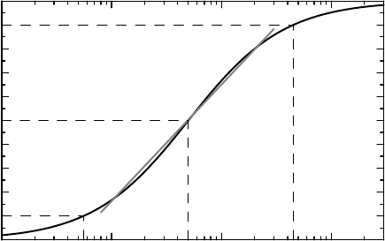
. The graph of a typical dose–response

function is shown in Figure 10.1.

In many situations it is useful to think of the dose–response relationship in terms of a

CDF of a stochastic variable. For example, we may think of a painkiller drug as a drug that

blocks pain mediating neurons. More neurons can be blocked with more drug in the body. We

can think of F (D) as the proportion of neurons blocked when the subject is given the dose

D. What we measure is the subjective pain realized by the patient. Denote the no-drug pain

level by P

and assume that very large doses can reduce it to zero (all neurons are blocked).

The pain that is experienced when a subject is given the dose D is then described by the

function G(D) = P

(1 − F (D)), but to be consistent with assumption 2 above (an increasing

dose–response relationship) we measure the effect as E(D) = P

− G(D) = P

F (D).

DOSE–RESPONSE RELATIONSHIP 275

0.1

0.2

0.3

0.4

0.5

0.6

0.7

0.8

0.9

Normalized response

Dose (on log-scale)

Figure 10.1 A typical dose–response curve and the log-linear approximation with ED

well as ED

and ED

indicated.

Another example is a β

-agonist taken by a patient with asthma when he has difﬁculty

breathing. The action of the drug is to relax muscles in the lung, so we can think of F(D)

as the proportion of contracted cells that have been relaxed when dose D is given. The lung

function is measured by a variable such as FEV

.IfE

is the value of FEV

when all the

relevant muscles are contracted, the FEV

measurement (which is a response, not an effect),

as a function of dose, can be written as a function R(D) = E

+ E

max

F (D). Here E

+ E

max

would mean the level of FEV

that is obtained when all the contracted muscles are relaxed.

The actual effect of the drug is given by the function E

max

F (D).

Both these examples illustrate an important aspect of dose–response relationships – it

does not need to be the same on different occasions, not even for the same patient. In the last

example, the extent to which the muscles have been contracted may differ between occasions,

and values of E

and E

max

may differ between occasions. It may be that E

+ E

max

is relatively

ﬁxed for the individual, but E

varies as the pre-treatment proportion of contracted muscle

cells vary. If we assume that E

+ E

max

is constant, this means that the room for improvement

depends on the baseline conditions, and these are in turn are intimately connected with the

study design, in particular the choice of inclusion criteria for patients to be entered into the

study, and on what background medication the study will be carried out.

There is one further aspect of dose–response functions illustrated in Figure 10.1 – they

are often almost log-linear over a range of doses. This means that

E(D) ≈ α + β ln D

in some dose range, expected to be symmetric around ED

on the logarithmic scale. This is

consistent with the medical tradition of increasing doses by doubling when there is insufﬁcient

effect. The parameter β measures how sensitive the response is to changes in the dose. For

example, doubling a dose means an increase in response of size β ln(2) ≈ 0.69β.

The dose range over which the log-linear approximation of the dose–response curve is

reasonably accurate is the range over which the interesting doses can be found. Smaller doses

have only minute effects, and increasing the dose above the upper limit of this interval does

not give any measurable further increase in effect. This dose range may be deﬁned by ED

276 ANALYSIS OF DOSE RESPONSE

and ED

, and when we study doses in this dose range, the log-linear model should sufﬁce

for all practical purposes.

The consequence of this observation about log-linearity is that we can write the general

dose–response function as

E(D) = E

max

(a + b ln D),

where a and b are parameters, and (x) is some CDF such that (0) = 1/2, and which is

almost linear on some interval around x = 0. The condition (0) = 1/2 is only a convenient

normalization, and implies that ln ED

=−a/b. The constant b measures the sensitivity to

the drug, but is not the same as the β above. (To relate the two, note that the slope of the tangent

at the ED

point in Figure 10.1 is given by bE

max





(0), which is therefore an approximation

to β.)

The most popular choices for the distribution function (x) are the two related CDFs

discussed in Box 9.4, the standard Gaussian distribution (x) = (x), and the logistic distri-

bution (x) = (1 + e

−x

)

−1

. In the logistic case we get the explicit and much used expression

(a + b ln D) =

+ D

This model is often referred to as the Emax model, and the coefﬁcient b is called Hill’s

coefﬁcient, named for the English statistician A. V. Hill.

Example 10.1 In a typical experiment in toxicology, increasing doses/concentrations of a

chemical are given to groups of mice, and the number of deaths is counted. In one experiment,

in which each dose group consisted of 10 mice, the following data were obtained:

dose: 5 25 100 800

deaths: 1 3 8 10

For each dose level D there is a probability p(D) of death for a mouse given that dose. This is

true for all doses; what is particular with the doses we actually study is that for them we can

estimate these probabilities. However, we want to use this information to interpolate between

doses in order to be able to estimate ED

. This is the dose that kills 50% of the mice and

is called LD

, where LD stands for lethal dose. To estimate LD

we need a model for the

dose–response relationship.

If we model the probability of death as a function of dose, by using the function

p(D) = (a + b ln D) with the logistic CDF (x), we have that

p(D)

1 − p(D)

= a + b ln D,

where the left-hand side is the log-odds for a mouse death at dose level D. This is a logistic

regression model with the log-dose as covariate. Analysis of the data gives us the parameter

estimates a =−4.95 and b = 1.36. From this we can estimate the lethal dose for 50% of the

animals, which is given by the formula LD

= exp(−a/b), as 37.6 with 95% conﬁdence

limits (18.4, 76.9). Here we have used Fieller intervals to obtain the conﬁdence limits for the

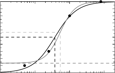
ratio a/b and then exponentiated the result. The predicted dose–response curve is shown in

Figure 10.2 as the black curve, and LD

is indicated by a dashed (black) line.

DOSE–RESPONSE RELATIONSHIP 277

0.1

0.2

0.3

0.4

0.5

0.6

0.7

0.8

0.9

Percent mice dead

Dose of drug

Background mortality

Figure 10.2 Two models for a toxicology experiment. The original model is in black, the

modiﬁed one that takes background mortality into account is in gray.

However, the fact that we had a death in the lowest dose group raises the question whether

there was some background mortality that needs to be taken into account when we model the

dose response. The experiment was therefore repeated on another batch of 20 mice, except

that these did not receive the chemical. It turned out that 3 out of these 20 animals died. It

was therefore decided that a background mortality needed to be incorporated into the model,

which we can do by writing it as

p(D) = π + (1 − π)(a + b ln D).

Here π is the probability that an animal dies during the experiment for reasons independent of

the chemical, and the function (a + b ln D) now describes the excess risk, which is what we

want to relate LD

to. The estimation of these parameters is easily done by use of the GLS

method discussed in Section 9.3. The resulting parameter estimates are a =−8.16, b = 2.05

and π = 0.13, and from this we obtain the estimate 53.6 with 95% conﬁdence limits (25.6,

111.5) for LD

. Figure 10.2 shows the resulting dose–response curve in gray. Again the

value is indicated by dashed (gray) lines. The corresponding level is greater than 0.5,

which illustrates that in this case LD

does not correspond to an observed count of 50%

dead mice, but to an observed count of 57% dead mice, since 0.13 + 0.50(1 − 0.13) = 0 .57,

accounting for natural mortality.

The assumption that the dose–response curve is an increasing function of the dose may not

always manifest itself in data, because other factors may start to take effect at higher doses. It

may be that the ability to perform the outcome measurement is impeded by some drug-related

side-effect; if the drug causes headache the patient may not fully appreciate the improvement

in the symptoms of the disease without the headache, despite the fact that the headache has

nothing to do with the disease symptoms. If we need to model such complicated aspects of

the readouts we may want to subtract, from the strictly increasing function discussed above,

another function which starts to take effect at higher doses and describe these other effects,

thereby obtaining a dose–response curve that is not increasing over the whole dose range. This

leads to more parameters to ﬁt, and we should be very conﬁdent that this is the appropriate

278 ANALYSIS OF DOSE RESPONSE

model to use before applying it. That a mean was observed to be lower for a higher dose, as

compared to a lower dose, is not sufﬁcient evidence that this is also true for the underlying

true means.

10.3 Relative dose potency and therapeutic ratio

Before we take a closer look at the estimation problems related to dose–response relation-

ships, we consider what we wish to describe with such an analysis. One investigation of

interest is to compare the dose–response relationship for two different drugs on the same

outcome variable(s), another to compare the dose–response relationships for two different

outcome variables for the same drug. We may even want to compare a number of differ-

ent outcome variables for two different drugs. Similarly to what we did when we compared

distribution functions in terms of distributional parameters, we need to ﬁnd simple ways to

summarize and communicate the result.

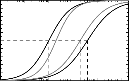
Figure 10.3 illustrates the main issues in dose–response modeling, at least in drug

development. We have two drug treatments, denoted A and B, and for each of these the

dose–response relationship for two different outcome variables. One represents a positive

effect, the other a side-effect. Inspecting the graph, we see that for the (positive) effect we have

= 10 for A and ED

= 20 for B. In comparative terms we can say that the relative

potency, ρ = ED

(B)/ED

(A), is 2 for A versus B.(A is more potent since its ED

is smaller.) The number ln ρ is the horizontal distance we need to move the dose–response

curve of B to the left, in order for it to pass through the ED

for A. It is important to plot the

response curve versus dose on a log scale for this in order to assess the extent to which such

a description conveys the important features of the situation at hand. In Figure 10.3 the dose

sensitivities (the slopes of the curves) of the two treatments differ slightly, so this shift will

not put the entire dose–response curve for B on top of that of A. If the outcome has the same

dose sensitivity to the two drugs, this is what would happen, and in such a case the difference

0.1

0.2

0.3

0.4

0.5

0.6

0.7

0.8

0.9

Fraction of maximal effect

−1

Dose of drug

eff

−

eff

−

eff

Figure 10.3 Geometric description of the relative dose potency and the therapeutic ratio for

two drugs. Drug A is shown in black, drug B in gray. The positive effect is represented by the

pair of curves on the left, the side-effect by the pair on the right.

SUBJECT-SPECIFIC AND POPULATION AVERAGED DOSE RESPONSE 279

between the two drugs would be completely described by ρ – drug A is twice as potent as

drug B. With different dose sensitivities the picture is more complicated, but as a ﬁrst approx-

imation this description may still be a reasonable summary. This is the same situation as when

we compare the means or medians for two distributions that are not true horizontal shifts of

each other.

Next we consider the side-effect, for which the difference in sensitivity is smaller. Again it

is reasonable to express the difference between the two treatments as the relative potency, and

we ﬁnd that ρ = 0.5, since the ED

is 400 for A and 200 for B. If we look within treatment,

we have that the ratio of the ED

for the effect to the side-effect is 400/10 = 40 for A;it

is 40 times more potent on the effect side than on the side-effect side. We call this ratio the

therapeutic index.ForB we calculate this number to be 10. The ratio of these therapeutic

indices constitutes the therapeutic ratio for A versus B, found to be 4 in our case. This means

that, in some sense, A is four times better than B at separating positive from negative effects.

The therapeutic ratio can also be written as the ratio ρ

/ρ

−

, where ρ

(ρ

−

) is the relative

potency for the two drugs on the positive effect (side-effect). We can therefore compute the

relative dose potency for the two drugs for the effect and side-effect separately, and form this

ratio to obtain the same parameter (in this case 2/0.5 = 4). As a summary measure this is

most useful if the dose–response curves are parallel shifts of each other for the positive effect

and for the negative effect separately, but the two outcomes need not have the same dose

sensitivity within drug.

10.4 Subject-speciﬁc and population averaged dose response

So far we have discussed the shape of a single dose–response curve. When we study dose–

response data from many subjects, we encounter a particular problem, namely that dose–

response curves may differ between individuals, and between occasions for individuals. This

means that we should expect heterogeneity in the response curve, which is a problem equiv-

alent to that of the omitted covariates in Section 9.6; what is the dose–response function here

was the response function there. The present discussion is therefore a further illustration of

what was discussed back then.

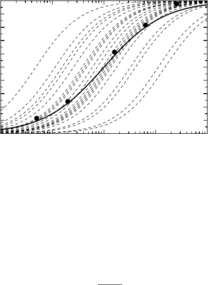
The problem is illustrated in Figure 10.4 in a very simpliﬁed setting. The assumptions

underlying this graph are as follows. We study an outcome variable for which the minimum

and maximum levels are well deﬁned, so we can normalize these to zero and one. We also

assume that the sensitivity to the drug is the same for all individuals; what differs is the dose

required to achieve a certain effect. More speciﬁcally, we assume that the dose–response curve

for an individual is given by the simple formula

E(D) =

θ + D

where the parameter θ = ED

varies in the population according to some distribution with

CDF P (θ), which we take to be lognormal for our discussion. We have a sample of 20 such

dose–response curves, shown in Figure 10.4 as the dashed curves. Each of these is (on the

logarithmic dose scale) a translated version of the one deﬁned by θ = 1.

The solid curve in Figure 10.4 represents something different. It is the average of all

responses at given doses, that is, the population mean values of the outcome variable at a

given dose. This curve has a slope which differs signiﬁcantly from that of the individual

280 ANALYSIS OF DOSE RESPONSE

0.1

0.2

0.3

0.4

0.5

0.6

0.7

0.8

0.9

Fraction of maximal effect

−2

−1

Dose of drug

Figure 10.4 The difference between subject-speciﬁc curves and the population average

curve. The dashed curves shows a sample of dose–response functions for different individuals,

whereas the thick curve is the population average. The dots represent mean values for selected

doses from the individual curves plotted with a measurement error added – see text.

curves. Mathematically the solid curve is obtained as the average over the population of the

individual dose–response curves, and is given by the formula

E(D) =



∞

−∞

θ + D

dP(θ).

(We referred to this graph in Section 9.6, where the dashed curves were logistic functions

for different values of the missing covariate Z, and the solid curve is the average response

function for the population.)

In order to describe the dose response in a population we therefore need to decide what it

is we wish to describe:

1. The individual dose–response functions are referred to as subject-speciﬁc functions.

These are usually described by a family of functions f (θ, D) which depend on some

parameters θ and on the dose D. What varies in the population is θ, according to a

CDF P(θ), and when we wish to describe the subject-speciﬁc dose response we need

to identify the functions f (θ, D) and P(θ).

2. The population averaged function, on the other hand, is a single function which, for

each dose, describes the mean effect in a population when that dose is given to all

subjects. In this case there is only one regression function we need to identify.

The regression function may well depend on covariate information; we may, for example,

wish to identify different dose–response functions for males and females.

For our example, the subject-speciﬁc description is that the dose–response functions take

the form E(D) = D/(e

+ D), where ξ has a Gaussian distribution with mean zero and

variance σ

= 2. The population averaged dose response, on the other hand, turns out to

ESTIMATION OF THE POPULATION AVERAGED DOSE–RESPONSE RELATIONSHIP 281

be well approximated by the function

E(D) =

3/4

1 + D

3/4

(This result was obtained from a nonlinear regression analysis, but if we replace the logistic

function with a Gaussian CDF we can repeat the argument in Example 9.6 to ﬁnd b = 0 .769,

which therefore should be a good approximation.)

Which of these two descriptions of the dose response is the most appropriate depends on

how we want to use the information. If we want to use it to choose one or more doses to develop

further in a drug development program, for ultimate use in the clinic, the population averaged

approach seems to be the most appropriate. If, on the other hand, we want a personalized

medicine approach and want to introduce a method to decide on the individual dose for each

speciﬁc patient, we may want to estimate that subject’s dose–response curve and how his

parameters depend on measurable covariate information.

One further complication is that when we actually measure the outcome, these measure-

ments will probably include observation errors. The observed measurements will therefore

not be found on the subject-speciﬁc curve, but scattered around, as deﬁned by some random

noise. This is illustrated in Figure 10.4 by the point marks, which represent the observed

mean values for a few doses. These are obtained from the 20 dose–response curves displayed

in Figure 10.4, but where to each observation we have added a measurement error with a

Gaussian distribution with zero mean and standard deviation 0.1. Note that we sampled 20

subjects and measured their response on ﬁve different doses, as opposed to having sampled

100 different subjects, on each of which we have measured the response to one single dose.

The issue illustrated here is not conﬁned to dose response, nor to experimental studies for

that matter. In epidemiology it is important to make a clear distinction between cross-sectional

and longitudinal studies. Take growth as an example. When puberty sets in, there is ﬁrst a

short-lived reduction in growth rate, followed by a growth spurt which slowly ﬂattens out as

the child approaches ﬁnal height. This is clearly seen when we investigate the growth curve

for individual children. However, puberty occurs at different ages for different children (and

earlier in girls than in boys), which means that if we measure height in a cross-sectional study

(sampling individuals more or less at a random age) and plot the mean height versus age from

such data, we may ﬁnd a smoothed curve with no distinct puberty-related effect.

10.5 Estimation of the population averaged dose–response

relationship

In this section we will illustrate the discussion in Section 9.5 by showing how to estimate the

population averaged dose–response relationship. Suppose we have obtained, possibly from

an earlier analysis, estimators ˆm

for the population mean response m

when the patients have

been given dose D

, i = 1,...,d, and that these estimates have a Gaussian distribution such

that ˆm ∈ AsN(m, ). Here m = (m

,...,m

) is the vector of mean responses (the points

in Figure 10.4) and  is the covariance matrix for the corresponding estimator, which may

depend not only on m but also on some auxiliary parameter φ. In the common case where

adjusted means were obtained from a linear model with a Gaussian error distribution, we have