Kallen A. Understanding Biostatistics

Подождите немного. Документ загружается.

292 HAZARDS AND CENSORED DATA

intuitively ‘intensity’ is more neutral, whereas ‘hazard’ is associated with risks). We take a

deterministic view and assume we have a very large population for which a function F (t)

describes the fraction of individuals who have experienced the event up to time t (the CDF

for the corresponding stochastic variable). The (possibly time-dependent) intensity function

λ(t) for this event is deﬁned by the differential equation (see also Section 2.7)



(t) = λ(t)F

(t).

In words, the rate at which new events occur in the population is proportional to the number

of individuals who have not yet experienced it, that is, the population still at risk. We assume

that an individual only can experience the event once. If we use the fact that F

(0) = 1, high-

school calculus shows that F

(t) = e

−(t)

, where (t) =



λ(s)ds is the cumulative intensity

(or hazard) function. The cumulative intensity (t) relates to the intensity λ(t) in the same

way as the CDF relates to the probability density.

We can write the differential equation above in the notation of Box 4.8 as

dF (t) = F

(t−)d(t), (11.1)

noting that the proportion at risk at time t is actually the left-hand limit F

(t−). At a jump

point of F (t) the relation, expressed as probabilities, reads

P(T = t) = P(T ≥ t)P (T = t|T ≥ t),

which means that the hazard d(t) = P(T = t|T ≥ t) is the conditional probability that we

have a jump at time t, given that it has not yet occurred. This observation helps us also

to understand the meaning of the hazard d(t) at points where F (t) is continuous, as the

instantaneous conditional probability that the event occurs now, given that it has not yet

occurred. Equation (11.1) therefore means that the jump size at time t is the product of the

number at risk and the hazard at that time.

From equation (11.1) we learn how to obtain F (t) from (t). For smooth functions this

is the differential equation mentioned above; in the general case we integrate the expression

to get an integral equation for F (t). We will discuss this integral equation and its connection

to the Kaplan–Meier estimate of the CDF further in Section 11.8.

More important at this point is that we have the relation d(t) = dF (t)/F

(t−). If we

multiply the numerator and denominator on the right-hand side by the sample size, this means

that d(t) = dN(t)/Y(t), where N(t) is the expected number of events that have occurred at

time t and Y(t) the expected number at risk at the same time t. This immediately leads us to

the Nelson–Aalen estimator 

(t) of the cumulative hazard from the relation

d

(t) =

(t)

where N

(t) is the (cumulative) number of observed events at time t and Y

(t) the number ob-

served to be at risk for experiencing an event at the same time. Since d(t) is an instantaneous

probability, we can compute it from only those we observe, as long as we adjust N

(t) to mean

observed events only. This estimates the true hazard as long as any censoring mechanisms

operating are not related to the event we observe (more on this in the next section).

HAZARD MODELS FROM A POPULATION PERSPECTIVE 293

Box 11.1 The Gompertz distribution

A survival distribution much used to describe life expectancy in insurance contexts is

a distribution which was introduced in 1825 by Benjamin Gompertz in an article with

the title ‘On the Nature of the Function Expressive of the Law of Human Mortality’.

The distribution is motivated by assuming

the average exhaustion of a man’s power to avoid death to be such that at the end

of equal inﬁnitely small intervals of time he lost equal portions of his remaining

power to oppose destruction which he had at the commencement of these intervals.

This assumption leads to the differential equation

λ(t)

−1

=−bλ(t)

−1

(where t is age) which is equivalent to the simpler equation λ



(t) = bλ(t), and implies

that λ(t) = λe

. The corresponding distribution is a generalization of the exponential

distribution (which is the case b = 0); when b/= 0 the survival function is given by

(t) = e

−λ(e

−1)/b

There is a connection between this distribution and the logistic distribution in

Box 9.4, via the generalized logistic function deﬁned by



(t) = F (t)(1 − F (t)

)/ν,

with ν is a further parameter. If we let ν → 0, this equation becomes F



(t) =

−ln(F (t))F (t), the solution of which is the Gompertz function.

In 1874 W.M. Makeham expanded this to a distribution with one additional param-

eter, deriving what is known as the Gompertz–Makeham law of mortality, which states

that the death rate is the sum of an age-independent component (the Makeham term) and

an age-dependent component (the Gompertz function). This appeared to be particularly

suitable as an approximation to many empirical life tables and therefore soon became

an important tool in actuarial theory.

The parametric distributions F (t) that appear for time-to-event data are typically not the

same as those that appear in the analysis of other types of measurement data. The Gaussian

distribution is usually not relevant here, being too symmetric for most applications, but the

lognormal distribution is a candidate, at least in some situations. However, it has a long right-

hand tail, and for this type of data, in particular mortality data, tails are often to the left instead,

which calls for a different set of distributions.

It is natural to derive the relevant distribution from the behavior of the intensity

function. The simplest case is when there is a constant intensity λ, so that (t) = λt and

F (t) = 1 −e

−λt

. In such a case T has an exponential distribution with parameter λ, denoted

Exp(λ) (the same as (1, 1/λ)). Like the lognormal distribution, it has a long tail to the right. Its

mean value is 1/λ and the graph of the function (t) is a simple straight line through the origin

with slope λ. It has the important and interesting property that it has no memory. This means

294 HAZARDS AND CENSORED DATA

(a) (b)

Hazard

43210

Time

0.2

0.4

0.6

0.8

Survival Function

43210

Time

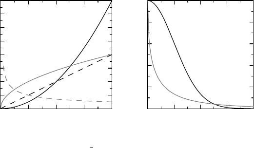
Figure 11.2 Illustration of the Weibull distribution. Dashed curves in (a) are graphs

of the hazard functions t and 1/

√

t, corresponding to Weibull distributions with ex-

ponents γ = 2 > 1 (black) and γ = 0.5 < 1 (gray), respectively. Solid curves in (a)

are the corresponding cumulative hazards, and the corresponding survival functions are

shown in (b).

that if the event has not occurred at time s, the time that remains until it occurs has the same

distribution as it had from the start; the distribution is insensitive to when we start our clock.

It is the only continuous distribution with this property. (In fact, since P(T>t+ s|T>t) =

(t + s)/F

(t), the ‘no-memory property’ is equivalent to the functional equation

(t + s) = F

(t)F

(s), for which the only (admissible) solution is F

(t) = e

−λt

.) This

property and the constancy of the intensity say the same thing: events occur completely at

random. So, when events occur completely at random, the time-to-event distribution is the

exponential distribution.

There are different directions in which we can generalize the exponential distribution

for time-to-event data. One such direction is the gamma distribution, which occurs when

there is a series of p events that build up the ﬁnal event, and the times between individual

sub-events are independent with a common exponential distribution. Another general-

ization is the Weibull distribution (Figure 11.2), which we write Wei(λ, γ). Compared

to the exponential distribution it has an additional exponent γ on the time variable,

so that

(t) = e

−λt

,(t) = λt

The corresponding hazard λ(t) = λγt

γ−1

is increasing with time if γ>1 and decreasing with

time if γ<1. The Weibull family of distributions constitutes a ﬂexible family for data when

one wants to understand how ‘non-exponential’ a particular distribution is. Furthermore,

P(ln T>t) = F

) = e

−λe

γt

and this distribution of ln T is called the smallest extreme value distribution. We will see

later that some important models for time-to-event data (AFT models) are actually regression

models for ln T , which explains why this observation is important.

We close this section with a description of the likelihood for a parametric model for time-

to-event data in the presence of right-censoring. We want to express the likelihood in the

HAZARD MODELS FROM A POPULATION PERSPECTIVE 295

Box 11.2 The likelihood for parametric hazard models with right-censored data

In order to compute the likelihood for a parametric model for continuous survival data in

the presence of right-censoring, let F

(t, θ) = e

−(t,θ)

where (t, θ) is the cumulative

hazard for λ(t, θ). For complete data the likelihood is given by

L(θ) = dF (t

,θ) ...dF(t

,θ) = λ(t

,θ) ...λ(t

,θ)F

,θ) ...F

,θ),

where t

is the observed event time for subject i. If we also have another m observations

about which we only know that they are larger than τ, for a ﬁxed number τ, then we

multiply this likelihood by F

(τ, θ) a total of m times. The resulting likelihood can be

written as

L(θ) =



λ(t

,θ)

,θ),

where δ

= 1 if this is an event (t

≤ τ) and δ

= 0 if the observation is censored and

we have that t

= τ for censored observations.

We now introduce a right-censoring process which is independent of the survival

time and with CDF C(t) and intensity function μ(t) not containing θ. What we observe

is the minimum of the time to event and the time to censoring, so what we observe

has a CDF Q(t, θ) which is such that Q

(t, θ) = F

(t, θ)C

(t). The likelihood L(θ)

now becomes



λ(t

,θ)

μ(t

)

1−δ

,θ) =



λ(t

,θ)



μ(t

)

1−δ

The relevant (θ-free) part of the log-likelihood can therefore be written as

ln L(θ) =



(ln λ(t

,θ)N

(t) − (t

,θ)),

where we have written δ

as N

(t) instead. In integral notation this is equation (11.2).

intensity function instead of distribution function, in order to smoothly handle censoring. Let

λ(t, θ) be the intensity function. As is outlined in Box 11.2, we have that

ln L(θ) =



∞

ln λ(t, θ) dN

(t) −



∞

(t)λ(t, θ)dt, (11.2)

where N

(t) and Y

(t) are as before. To ﬁnd the maximum of this function, we differentiate.

The equation that determines the estimate of θ from data is then given by



∞

∂

λ(t, θ)

(dN

(t) − Y

(t)d(t, θ)) = 0. (11.3)

This equation will, in various forms, prove to be fundamental in the next chapter.

296 HAZARDS AND CENSORED DATA

11.4 The impact of competing risks

There is a special consideration for right-censored data which is not relevant to complete data,

namely an understanding of the censoring mechanism. We have already pointed out that the

Kaplan–Meier estimator estimates the CDF. Its use may be uncontroversial if we are studying

time to death and a data point is censored for an individual only when he has yet to die. If,

however, we want to study mortality in a particular disease, it is a complicating factor that

patients may die from other causes. It may be that understanding time to death in the particular

disease is what is important to the investigator, because that is what a particular treatment

targets, but from the patient’s perspective the situation may be different. He may want to learn

how much longer he is expected to live if he takes the treatment, especially if there is a price

for taking it, such as side-effects. It is also possible that there are some negative effects of a

treatment, which leads to an increased mortality in other diseases, such as heart attacks. The

cause of death may be less important to the patient.

Suppose we are studying a particular event, such as death in a speciﬁc disease, in the

presence of competing events which, when they occur in an individual, do not allow us to

study the event we are interested in. What we can always estimate is the function G(t), which

is the probability that an event has occurred by the time t (it has occurred in the interval (0,t]).

It is simply the proportion of individuals for whom this event has occurred, and is called the

cumulative incidence function (CIF) for the event. It is not a distribution function, since in

the presence of competing risks we expect to have that G(∞) < 1. But it has all the other

properties of a CDF, and is therefore called a sub-distribution function. If we denote by T the

time we can observe, which is when the ﬁrst of the competing events occurs, the following

relation holds:

dG(t) = P(T

= t|T ≥ t)P(T ≥ t),

where T

denotes the time to the event we are interested in. If F (t) is the CDF for T , this

relation can be written as

dG(t) = F

(t−)d

∗

(t)

where d

∗

(t) is the event intensity among those that have not experienced any event yet. This

is not the same as the hazard d(t) deﬁned earlier, which is associated only with the event.

The hazard d

∗

(t), on the other hand, is very much deﬁned by what competing risks operate,

because it measures intensity on patients who so far have survived these. When we eliminate

one particular risk, it is not necessary that the hazards for the remaining ones are unchanged.

If we take away a risk factor for a particular cause of death, we may well affect other causes

as well: tobacco smoking not only induces lung cancer but also has effects on cardiovascular

death risks, as well as on other causes of death. If we give a drug that reduces blood clotting

we may reduce the risk of cerebral infarction, but increase the risk of cerebral hemorrhage,

leaving the overall risk of dying from a stroke unchanged.

We can estimate d

∗

(t) by the Nelson–Aalen ratio of number of observed events divided

by number at risk for this. The question then is when this estimates d(t), so that we can

deduce the CDF for the time variable we are interested in. This question assumes that there

is a well-deﬁned stochastic variable T

, free of the environment, that we can discuss. This is

not necessarily the case.

THE IMPACT OF COMPETING RISKS 297

Example 11.2 Suppose we are studying a chronic but ﬂuctuating disease for which there

naturally occur periods of symptom worsening, so-called exacerbations. Our treatment is

expected to reduce the intensity of the occurrence of such exacerbations, and we have a

placebo control. As part of the protocol the patient is allowed to discontinue participation in

the study whenever he wishes, and in doing so he should state his reasons for discontinuation.

One such reason may be a deterioration of the disease under study. Even though such a

withdrawal is not an exacerbation per se, not fulﬁlling the precise medical criteria for this, it

may well be closely related to it. It may, for example, precede it. If we study the time to the ﬁrst

exacerbation and censor these withdrawals, we probably will not do a meaningful analysis. It

may be better to redeﬁne the event under study as either exacerbation or discontinuation due

to deterioration of the disease.

If the variable T

exists, we have that d(t) = P(T

= t|T

≥ t). We can only measure

d

∗

(t), which works conditionally on T ≥ t, so if we want to substitute d

∗

(t) for d(t), we

need the cause-speciﬁc hazard to stay the same if we remove subjects experiencing competing

events. Essentially that means that our event and the competing events must act independently

of each other.

This, like the ITT analysis we discussed in Section 3.7, is something that is often dif-

ﬁcult for medical researches to accept: ‘why can’t I analyze non-fatal and fatal myocardial

infarctions separately?’ The answer is that even though it may make medical sense to do this,

there is simply not enough data to do a valid statistical analysis. Instead we need to make

a fundamental assumption, that competing risks act independently of the event of interest,

so it is the shortcomings of statistics (or, rather, the amount of information) that hinder the

fulﬁllment of this wish.

If we can somehow assume independence, we can estimate (t) from data, considering

those individuals with a competing event to be censored, and thereby obtain the Kaplan–Meier

estimate of the CDF for T

. It may also be that we want to eliminate only some censoring

reasons. Suppose we are studying the events ‘death from myocardial infarction’ and ‘death

from other causes’, but also that patients in the study may be lost to follow-up. In order to be

able to estimate the CIF for death from myocardial infarction in the presence of other causes

of death, we want to eliminate the problem posed by those who were lost to follow-up and to

study termination. This is done by use of the formula

G(t) =



(s−)d(s),

where d(t) is cause-speciﬁc and is estimated from the Nelson–Aalen estimator, and F

(t)

is estimated by the Kaplan–Meier estimate for total survival. In this way we get an estimate

of the CIF, eliminating the study-speciﬁc censoring mechanisms.

One lesson from this discussion is that the Kaplan–Meier estimate relates to an abstract

time-to-event variable, free of any competing events. To describe the results of an analysis

in terms of the Kaplan–Meier estimate may therefore be somewhat artiﬁcial in situations

where there are competing risks that cannot be eliminated. In such a situation it may be more

relevant to compute something like the function G

(t)/G

(t). This represents the conditional

probability for the event prior to time t, provided that the none of the competing risks have

yet occurred. This is how the Kaplan–Meier estimate is sometimes (erroneously) interpreted.

The Kaplan–Meier estimate is an estimate of the CDF for the event in the absence of other,

competing, events. The suggested function provides the probability of obtaining an event of

298 HAZARDS AND CENSORED DATA

Box 11.3 Bernoulli’s model as differential equations

Bernoulli’s analysis did not discuss vaccination against smallpox, since Edward Jen-

ner’s work on inoculation with cowpox was still 30 years in the future. Instead it was

concerned with variolation, in which infectious material is inoculated into the skin of

the susceptible in order to induce a mild infection. This was not an altogether harmless

process; children could die from it, and it could trigger small epidemics. At the time

physicians argued about whether the beneﬁts of inoculation outweighed the risks, and

the objective of Bernoulli’s paper was to provide some numbers to facilitate decision

making. As such it is one of the earliest attempts at evidence-based medicine.

In his analysis Bernoulli used the then recently developed methods of calculus.

Introducing the two unknowns x(a), the number of susceptibles at age a, and n(a), the

total number surviving to age a, he wrote down the two differential equations



(a) =−(λ + μ(a))x(a),n



(a) =−pλx(a) − μ(a)n(a),

subject to the initial conditions x(0) = n(0) = n. Here λ is the force of infection, μ(a) the

age-dependent death rate, and p is the probability of dying from smallpox. From this he

derived the following differential for the prevalence f (a) = x(a)/n(a) of susceptibles:



(a) = λf (a)(pf (a) − 1),f(0) = 1,

which we solve to get f (a) = 1/(p + (1 − p)e

λa

). Bernoulli could then estimate the

number of deaths due to smallpox, and deduce that in an environment free of smallpox

the fraction surviving to age a should be given by e

λa

/(p + (1 −p)e

λa

). He described

the result of his investigation by adding new columns to Halley’s tables, containing

‘would-be’ data.

the type under study, given that a competing event has not occurred. It will depend on the

environment in which it operates.

The competing risk discussion is important when we try to assess what the overall effect

would be if we took action to modify one of the competing risks. What does the elimination

of one particular cause of death do to overall mortality? This may well be the relevant health

economic question for a new drug treatment, whereas the relevant biological question may

address what happens in an environment free of competing risks. The former type of question

was actually where the mathematical theory of competing risks started, and its history preceded

mainstream statistics when, in the mid eighteenth century, Daniel Bernoulli of the (among

mathematicians) famous Bernoulli family, wanted to understand what inﬂuence smallpox

had on overall mortality. The speciﬁc question he addressed was the following. Published

life tables reﬂect the mortality of the population for which they were calculated, taking into

account all causes of death, including smallpox. How would these life tables change if, because

of mandatory vaccination, deaths from smallpox were entirely eliminated?

We will address this question in a way similar to Bernoulli’s approach, but investigating a

probability model, where Bernoulli used differential equations. An outline of his approach is

given in Box 11.3. His calculations were based on a life table compiled in 1693 by the English

astronomer Edmond Halley (of Halley’s comet) from the records of the then German city of

Breslau (now Wrocław in Poland) on the age at death of each individual in the town.

THE IMPACT OF COMPETING RISKS 299

For a person who is alive and still susceptible to smallpox (i.e., has not yet been infected),

at age a, there are two competing risks:

1. He may contract smallpox, from which he dies with probability p(a). Let S(a) denote

the distribution for the age at which the subject contracts smallpox in an ‘environment

free of other causes of death’.

2. He may die for reasons unrelated to smallpox. Let H(a) denote the lifetime CDF in a

‘smallpox-free environment’.

Bernoulli’s objective was to estimate the survival function H

(a). His argument was essentially

as follows. Someone who is alive at age a either is alive and susceptible to smallpox, which

occurs with probability H

(a)S

(a), or has had smallpox, survived it and not yet died from

other causes. The probability of having contracted smallpox and survived to age a is given by



(1 − p(α))dS(α), from which we deduce that the overall probability of survival to age a is

given by

l(a) = H

(a)



(a) +



(1 − p(α))dS(α)



Note the independence assumptions here. The left-hand side is (approximately) provided by

Halley’s table, so we obtain the expression

(a) =

l(a)

(a) +



(1 − p(α))dS(α)

If we assume, almost certainly incorrectly, that the probability of dying from smallpox is age-

independent, p(a) = p, we can write this as H

(a) = l(a)/((1 − p) + pS

(a)). Bernoulli also

assumed that there is an age-independent risk λ of contracting smallpox, so that S

(a) = e

−λa

and therefore arrived at the expression

(a) =

l(a)

1 − p + pe

−λa

To obtain parameter values he assumed that during one year smallpox attacks one in eight

individuals, so that λ = 1/8, and that it causes death in one in eight who are infected,

so that p = 1/8 as well. Under these assumptions the eradication of smallpox would be

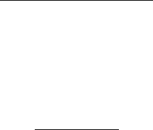
expected to increase the median age at death by 12.4 years from about 11.4 to 23.9 years,

which is illustrated in Figure 11.3. Under the model we can also compute the mean life

expectancy from Halley’s table, which predicts an increase of 3.1 years, from about 26.6

to 29.6 years.

As already noted, there are some strong assumptions in these calculations, an important

one being the independence between death from smallpox and death from other causes. But

this is a modeling exercise, and when we ﬁnally inspect the result and compare with our

predictions, we must bear in mind that this assumption may explain some of the discrepancy.

Likewise, when we discuss the modeling predictions we must assess how sensitive they are

to the assumptions, not only the independence assumption but also other assumptions made.

This makes modeling an endeavor with special problems, especially if you cannot test the

model before you need to make your decision. Climate modeling today is a case in point.

300 HAZARDS AND CENSORED DATA

0.4

0.5

0.6

0.7

0.8

0.9

20100

e (

ears)

Halley’s data

Bernouilli’s prediction

Figure 11.3 Life table data based on Halley’s data with and without smallpox. The gray

curve shows Halley’s tabulated data, the black curve Bernoulli’s prediction of how it would

change if smallpox were eradicated.

11.5 Heterogeneity in survival analysis

It is tempting to interpret the hazard, or the survival function, computed on population data

as individual risks. This is often not appropriate, basically because biological systems do

not consist of cloned, identical individuals living in identical environments; instead there is

biological variation. In fact, one of the purposes of a statistical analysis is to explain part of this

variation in terms of covariates. We have already seen that omitted covariates have different

effects in different statistical models. For some statistical models unobservable variation is

simply random noise with no effect on the size of the signal. This is true for methods such as

the t-test for means and ordinary linear regression. It is not true for time-to-event data because,

in a heterogeneous world, high-risk subjects will experience the event early and with time

we will gradually study more and more low-risk subjects. The hazard we see will therefore

decline with time because of a selection procedure, which may give us a false impression that

the individual hazards disappear with time. Although this may be true on a population level,

it may not apply on the individual level. Since the life expectancy is dependent on how frail,

or fragile, someone is, heterogeneity in this context is referred to as frailty.

To discuss this frailty problem we make a simple basic assumption about the nature of

the heterogeneity, which may or may not be realistic. At least it will help us understand

the problem and its consequences. The model in question, referred to as the frailty model,

assumes that individuals have proportional hazards, so that for each individual there is a

value θ, such that the hazard for that individual is given by θd(t), where d(t) is some

reference hazard, common to all individuals. The θ tries to capture the individual frailty,

which includes factors such as disease severity, genetic makeup or aspects of the (constant)

environment. We refer to the θs as frailties and assume that their distribution in the population

is described by a CDF P(θ). In order to be able to uniquely specify the reference hazard and

the frailty distribution, we assume that the latter has a known mean value. Let F (t) denote

the CDF corresponding to (t), and let F (t, θ) denote the CDF with cumulative hazard

HETEROGENEITY IN SURVIVAL ANALYSIS 301

Box 11.4 What can we deduce about frailty based on the outcome?

This box contains some mathematical details about the discussion on frailty the text.

If we randomly sample an individual from the population, the bivariate distribution

of the time-to-event variable T and the frailty θ has a density given by dF (t, θ)dP(θ).

The proportional hazards model means that

dF (t, θ)dP(θ) = [θF

(t−,θ)dP(θ)]d(t),

a relation that contains a lot of information. First, we can integrate out θ to obtain the

marginal density for T :

d(t) = S

(t)d(t), where S

(t) =



(t−,θ)θdP(θ).

Here F

(t−,θ)dP(θ) is the probability (density) that we get an individual with frailty θ

and for whom T ≥ t. It follows that F

(t−,θ)dP(θ)/

(t−) is the conditional density

for θ, given that T ≥ t, and therefore that S

(t)/

(t−) is the expected value of θ,given

that T ≥ t. The population hazard is therefore given by

d



(t) =

d(t)



(t−)

= E(θ|T ≥ t)d(t).

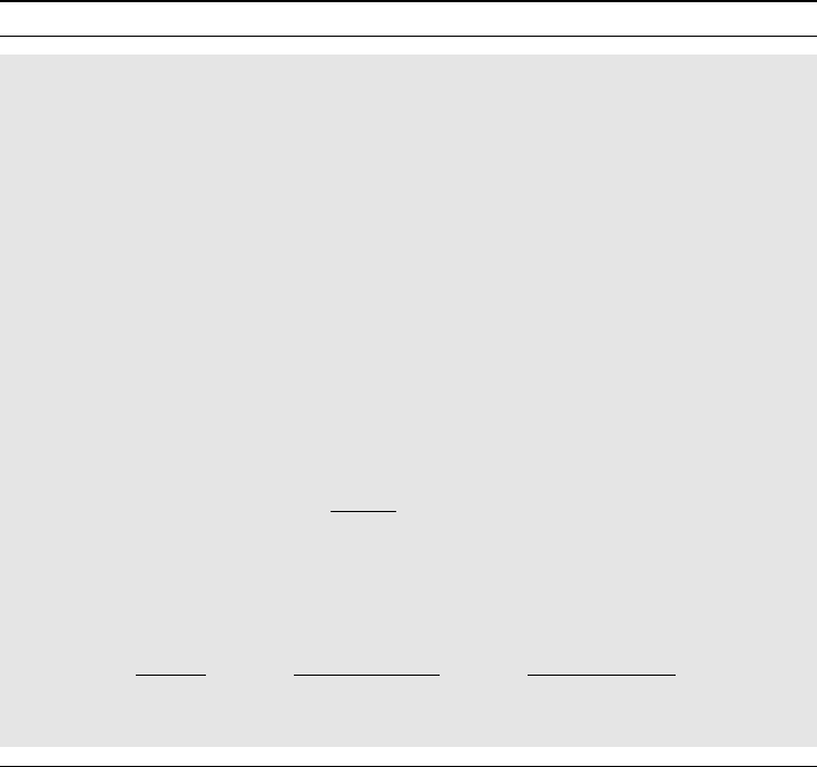
If we instead divide the bivariate density dF (t, θ)dP(θ) by the density d(t), we get

the conditional probability that the frailty is θ, given that we know that the outcome is

T = t. An alternative expression for this is obtained from above as

dF (t, θ)

d(t)

dP(θ) =

(t−,θ)θd(t)

(t)d(t)

dP(θ) =

(t−,θ)θdP(θ)

(t)

This is the density of the conditional frailty CDFs P(θ|T = t) shown in Figure 11.5.

function θ(t). Before proceeding, we note that the famous Cox model, which is so often

used in the analysis of survival data, has precisely this set-up, except that instead of a frailty

distribution it tries to explain the different frailties in terms of measured covariates. More

precisely, it assumes that there is a relation of the form θ = e

zβ

, where z are the covariates

and β are regression coefﬁcients that are to be estimated. This model is discussed in some

detail in Section 12.6 and our derivation of it will build on the observations we make in the

current section.

Now back to the basic setup. As seen in Box 11.4, we can derive some useful information

about the frailty of an individual based on knowledge about when his event occurred. The

marginal CDF for the time-to-event variable T is obtained by integrating θ out:

(t) =



F (t, θ)dP(θ).

This is the distribution we see in the population, and with some mathematical trickery, outlined

in Box 11.4, we can show that the corresponding population hazard is given by the expression

d



(t) = E(θ|T ≥ t)d(t).