Kallen A. Understanding Biostatistics

Подождите немного. Документ загружается.

302 HAZARDS AND CENSORED DATA

Box 11.5 Frailties with a gamma distribution

A popular choice for the frailty distribution P(θ) is the gamma distribution with mean

1 and variance 1/a. Its popularity is largely due to a simple Laplace transform:

L(s) =



∞

−sθ

dP(θ) = (1 +s/a)

−a

For a continuous variable, the population survival function for a frailty model is

given by



(t) =



−θ(t)

dP(θ) = L((t)).

For the gamma frailty case this implies that 

(t) = (1 + (t)/a)

−a

and that

d



(t) =

d(t)

1 + (t)/a

Since (t) is increasing, this means that the hazard ratio d



(t)/d(t) is decreasing

with time and the steeper (t) is (the more common the events) the greater is the role

played by frailty.

Consider an epidemiological situation where the baseline hazard is (t) for the

exposed, but r(t) for the unexposed, r<1. Assume that the heterogeneity is described

by the same gamma distribution for the two groups. If we denote by 

(t) the two

population hazards, we ﬁnd that

d

(t)

d

(t)

= r

1 + (t)/a

1 + r(t)/a

This instantaneous hazard ratio start out as r, but for very large t it approaches one.

The initial relative risk therefore seems to disappear. But this is only a reﬂection of the

fact that, for large t, we only study robust individuals for whom the event rarely occurs.

(With a different choice of frailty distribution we may even get a crossover, so that the

ratio approaches something greater than one.)

This qualiﬁes the intuitive discussion above, that the population hazard at time t is the mean

hazard, evaluated among the survivors. It is also time-dependent when the reference hazard is

constant, because what we know about the hazard at a later point in time is based on a selected

subgroup of individuals (those who survived that long) and not on all individuals. For more

on the important case where the frailty distribution is a gamma distribution, see Box 11.5.

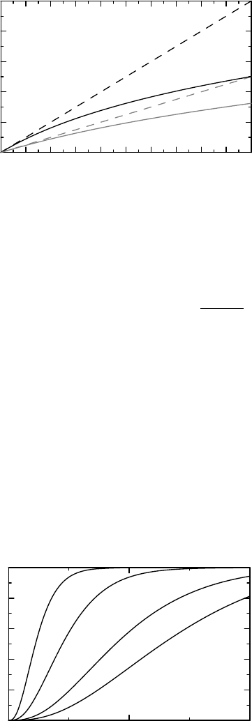
Example 11.3 Figure 11.4 is a graphical illustration of the consequences of the heterogeneity

for the cumulative hazard. We have two groups with constant hazards, one twice the other in

magnitude (dashed lines). These serve as (constant) baseline hazards in frailty models with

gamma-distributed frailties, with the corresponding population hazards shown as the solid

curves, matched by level of grayness. We see that the diverging baseline hazards get replaced

by population hazards that become parallel with time. The asymptotic vertical shift is easy to

HETEROGENEITY IN SURVIVAL ANALYSIS 303

Cumulative hazard

109876543210

Time (months)

Figure 11.4 The effect of population heterogeneity on survival and cumulative hazard

functions. The assumption is a gamma-distributed frailty distribution with variance one.

compute as

a ln(1 +(λt)/a) −a ln(1 + (λt/2)/a) = a ln



1 +

λt

2a + λt



≈ a ln 2.

In summary, in a world of frailty differences between people, the individual hazard may

look quite different from what we ﬁnd when we study a random sample from the population.

The proportional hazards model can be true on an individual level, but the marginal Kaplan–

Meier estimate may look quite different.

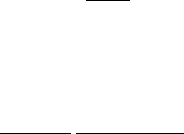
For the sake of completeness (and for other reasons which will become apparent at the end

of next chapter) we also want an expression for what we expect the frailty to be for a patient

for whom we have observed an event at time t. Box 11.4 also outlines how we can derive

the corresponding conditional frailty CDF P(θ|T = t), and these distributions are illustrated

in Figure 11.5, with similar assumptions as in the example above (constant baseline hazard

and gamma frailty). We see that P(θ|T = t) puts weight on smaller θ as t increases, which is

precisely what we should expect. This is generalized to the following statement about what

0.2

0.4

0.6

0.8

P(θ |T = t)

210

Frailty parameter θ

Figure 11.5 Illustration of the conditional frailty CDF P(θ|T = t) for some choices of t.

304 HAZARDS AND CENSORED DATA

we expect of the value of a covariate Z, given that we know that the subject had an event at

time t:

E(Z|T = t) = S

(t)

−1



E(Z|θ)F

(t−,θ)θdP(θ), (11.4)

where E(Z|θ) denotes the mean of Z for those subjects that have frailty θ. (For notation, see

Box 11.4.) This observation, together with the rest of the material discussed in this section,

will be important when we discuss the famous Cox model in the next chapter.

11.6 Recurrent events and frailty

In this section we digress a little from the main discussion on events that can occur only

once in an individual, and add a few comments about the case where there may be recurrent

events for individuals, bearing in mind that how prone individuals are to experience the event

may differ. Examples of recurrent events in biostatistics include the study of exacerbations of

chronic conditions such as asthma and other inﬂammatory diseases, epileptic seizures and the

recurrence of tumors. In such situations we may want to assess the event incidence by using

all observed events. The simplest way to do this is to reduce the data to the total number of

events for each individual, not concerning ourselves with when they occurred.

When we study individuals who can only experience a particular event once, for which the

(continuous) hazard is d(t), the process N(t) that counts the number of events can only

take on two values, zero (with probability e

−(t)

) and one (with probability 1 − e

−(t)

). If

there are recurrent events within subjects, and if we assume that all events are described

by the same hazard, the process that counts the events is a Poisson process (see Box 2.10),

so that N(t) ∈ Po((t)). Even if the exact conditions required are not necessarily fulﬁlled,

this may still be a reasonable description of the total count within a subject. However, there

are almost certainly different hazard functions for different individuals. As before, the frailty

model means that we assume that for each individual there is a θ such that N(t) ∈ Po(θ(t)),

and that θ has CDF P (θ) in the population. In order to compute the marginal distribution of

the number of events for individuals we ﬁx the time point t and write μ = (t). For a randomly

sampled individual the probability that precisely k events have occurred at time t is then

given by

p(k) =



∞

−θμ

(θμ)

dP(θ).

If we again consider the convenient case where the frailty distribution is gamma with mean

one and variance 1/a, we can compute this integral to obtain the probability function

p(k) =

(k + a)

k!(a)

(μ/a)

(μ/a + 1)

k+a

This is (see Box 11.6) the probability function for a negative binomial distribution with mean μ

and variance μ + a

−1

. The convention here is to call φ = a

−1

the overdispersion parameter,

since it inﬂates the variance (dispersion) compared to that of the Poisson distribution. When

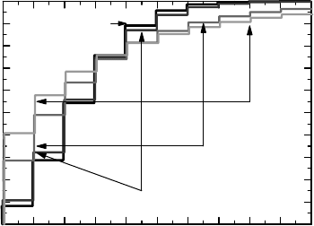
φ → 0 the negative binomial distribution becomes the Poisson distribution. To see the effect

of larger φ on individual probabilities, consider Figure 11.6 in which we compare the CDF

RECURRENT EVENTS AND FRAILTY 305

Box 11.6 The negative binomial distribution

To explain why the negative binomial distribution has this name, a small mathematical

tour is useful. The binomial theorem,

(1 + x)







holds true also when n is not a positive integer. For a positive integer n it shows that

with p = x/(1 + x) we have that



k=0





(1 − p)

n−k

= 1,

which deﬁnes the binomial distribution. Similarly, for n>0, but not necessarily

an integer,

(1 − x)

−n

∞



k=0

(−1)



−n



∞



k=0



n + k − 1



which leads us to the negative binomial distribution with probability function

(p = 1 − x)



n + k − 1



(1 − p)

Since p

(1 − p)

is the probability of k failures and n successes, if p is the probability

of success in identical and independent trials, this will be the distribution for the number

of failures until we have had n successes. The case n = 1 is the geometric distribution,

also called the binomial waiting time distribution, since it describes the number of trials

until the ﬁrst success.

The negative binomial is often parameterized in μ, where p = 1/(1 +μ). The

probability of k events is then given by



n + k − 1



(μ + 1)

n+k

and with this parameterization it can be shown that the mean is nμ and the variance

nμ(1 + μ).

for a Po(μ) distribution with that of a few negative binomials with the same mean, in order to

see the effect of the overdispersion. We see how the CDFs ﬂatten out as we increase φ, which

is what is to be expected: by increasing φ we introduce both more individuals with no events

and more individuals with many events.

One of the effects of using the negative binomial instead of the Poisson distribution is

therefore to increase the probability of no events. It could also be the case that a proportion of

the population cannot experience the event at all; they could be cured of the disease or immune

to it. It is not that they have a low intensity for the event, it simply does not happen to them.

306 HAZARDS AND CENSORED DATA

0.1

0.2

0.3

0.4

0.5

0.6

0.7

0.8

0.9

Cumulative probability

109876543210

Number of events

φ 0= .1

φ 1=

φ 2=

CDFPoisson

Figure 11.6 A comparison of the CDF for the Po(2.5) distribution (black) to that of the

negative binomial distribution with the same mean and a few choices of the dispersion

parameter φ.

The negative binomial does not fully capture this feature of two subpopulations (neither does

the Poisson distribution). For this we need a model with a CDF of the form p + (1 − p)F(x),

where p is the fraction in the subpopulation for which the event cannot occur, and F(x)isthe

CDF for the number of events for those that can experience it. In the case where F (x)isa

Poisson distribution, this is called a zero-inﬂated Poisson model.

In this discussion on recurrent events we have reduced data to a single within-individual

measurement, the total number of events per individual. This may not be what we really

want to do, but a more complete use of data requires more complicated methods. We will

address this problem in some detail in Section 13.4, where we will provide an example of the

application of this theory, and also carry the analysis further. The reason why we have chosen

to postpone giving an example comparing the Poisson and the negative binomial models will

then be clear – we want to introduce the so-called robust covariance estimate ﬁrst.

11.7 The principles behind the analysis of censored data

In order to analyze time-to-event data statistically we need to know more about their math-

ematical/statistical properties. We made a remark about the likelihood theory for parametric

models earlier; now we are interested in an analysis without parametric assumptions. The

actual analysis will be more extensively discussed in the next chapter when we not only com-

pare two groups, but also consider linear models for a proportional hazards model (the Cox

model). To carry this out, we need to understand not only how to obtain estimating equa-

tions, but also how to compute the corresponding variances. We therefore need to consider

time-to-event data in their proper mathematical context, which is different from that of other

data. As mentioned in the introduction, this is because we do not really observe an event time,

instead we repeatedly observe an individual and note, at each time point, whether the event

has occurred or not. The collection of such variables constitutes a stochastic process and (if

only one event can occur for each individual) this process can only transition from the state 0

to the state 1, which it does at the event time. Adding such processes for all individuals gives

THE PRINCIPLES BEHIND THE ANALYSIS OF CENSORED DATA 307

us a stochastic process which counts the total number of events that have occurred at each

time point. This puts this type of data within the framework of counting process theory.

For complete data we use the e-CDF F

(t) to estimate the CDF F (t). In order to understand

how good our estimate is, we investigate the difference F

(t) − F(t). For time-to-event data

the fundamental quantity is not the CDF, but the hazard d(t). We estimate it by the Nelson–

Aalen estimate, but in order to investigate how good such an estimate is, we look at the

difference F

(t) −



(t−)d(t). The expected value of this is zero, as can be seen from

an integration of the fundamental relation in equation (11.1). This becomes more convenient

if we multiply by the total sample size, so that this difference can be written as

ξ(t) = N

(t) −



(s)d(s).

As before, N

(t) is the total number of events that have occurred at time t and Y

(t)isthe

number of subjects at risk of an event at time t. The process {ξ(t); t ≥ 0}is simply the difference

between what we observe and what we predict from an assumption on the intensity d(t).

The process Y

(t)isapredictable process, which means that if we know its value just prior

to time t, what we expect next is precisely what we see now.

We can rewrite ξ(t) as an integral,

ξ(t) =



(dN

(s) −Y

(s)d(s)),

which means that it is a cumulative sum of components dN

(t) − Y

(t)d(t). Here

(t) is the rate of new events at time t, which we can think of as having a binomial

distribution Bin(Y

(t),d(t)). Its expected value is therefore Y

(t)d(t) and its variance is

(t)d(t)(1 −d(t)). For the variance, the last factor only comes into play if there is a jump

in (t), which means we can write it as Y

(t)(1 − (t))d(t). These observations imply

two important things:

•

The process ξ(t)isamartingale. Such processes are generalizations of cumulative (par-

tial) sums of small stochastic variables with mean zero, and are such that, conditionally

on what we know at time s, the prediction (conditional mean) for ξ(t) at a time t>sis

the present observation, ξ(s). In particular, the global mean is zero, since ξ(0) = 0.

•

The process

ξ(t) =



(s)(1 −(s))d(s)

takes on the role of a variance. Since it is a stochastic process, it is not the true variance,

but there is a CLT for martingales (described in Appendix 4.A and further explored in

Appendix 11.A) which asserts that it can be used for this very purpose.

There is one important observation more to be made. Test statistics are usually weighted aver-

ages of a predictable process {H(t); t ≥ 0}, weighted by the martingale {ξ(t); t ≥ 0}(weighted

averages of the differences between what is observed and what is predicted):

(t) =



H(s)dξ(s).

308 HAZARDS AND CENSORED DATA

Such a weighted process is also a martingale (use the fact that the conditional expectation of

dξ

(t) = H(t)dξ(t), given the state just prior to time t, can be computed by pulling H (t) out

of the expectation), and its variance process is given by

ξ

(t) =



H(s)

dξ(s) =



H(s)

(s)(1 −(s))d(s).

There now follow two important applications of this. The ﬁrst explains how the mathe-

matics works, when we derive information about right-censored processes.

Example 11.4 A censoring process C(t) is a predictable process which is one at time t if the

individual is observed, and zero otherwise. If N(t) is the number (zero or one) of events that

have occurred for an individual at time t, the number of observed events for that individual is

given by the integral



C(s)dN(s). Similarly, the number (zero or one) that are observed to be

at risk at time t will be C(t)Y(t). We then see that the process {ξ(t); t ≥ 0} above, which was

previously discussed in the absence of any censoring mechanism, has the properties stated

above also when N

(t) counts only the observed events and Y

(t) denotes the number observed

to be at risk.

Important special cases of the censoring mechanism are obtained as follows. A stochas-

tic time variable Z such that C(t) = I(Z ≥ t) is a censoring process is referred to as a

censoring time and corresponds to a right-censoring mechanism. More generally, we can

have two independent continuous stochastic variables, U, V such that 0 ≤ V ≤ U and deﬁne

C(t) = I(V<t≤ U). This is called Aalen ﬁltering and includes both right-censoring and

left-censoring as special cases.

The next example shows how we can obtain knowledge about (t) from the Nelson–Aalen

estimator 

(t). What we need is the variance of 

(t) − (t).

Example 11.5 For the Nelson–Aalen estimator we have that



(t) − (t) =



(s)

(dN

(s) −Y

(s)d(s)) =



dξ(s)

(s)

and since H(t) = Y

(t)

−1

is a predictable process, we have that the variance process for 

(t)

is given by



(s)

(s)(1 −(s))d(s) =



(s)

(1 − (s))d(s).

If we know that there are no jumps in (t), the immediate estimate of this is obtained by

replacing d(t) with d

(t). In the general case, recalling the discussion on page 158 on

estimation of the binomial variance, we obtain the tie-corrected variance estimate



(s) −N

(s)

(s) −1)

(s).

Note that when N

(t) = 1 the integrand reduces to the simpler expression dN

(t)/Y

(t)

Using this as a variance estimate, we can derive conﬁdence intervals for (t).

THE KAPLAN–MEIER ESTIMATOR OF THE CDF 309

The last observation in this example justiﬁes a quick discussion about ties for time-to-event

data. Even though there might be situations where the design of a study (or outcome variable)

is such that we could have pure jumps in the hazard, this is very rare. With continuous time we

therefore have that (t) = 0. However, we only measure time to a certain precision, such

as days. This means that two events that occurred at different time points may be recorded as

having occurred at the same time point. Had we measured to the precision of hours, many of

these ties would probably have been broken, and with more detailed timings even more so.

The proper way to handle ties that occur this way is to modify the Nelson–Aalen estimator to

account for what is really happening. In fact, if we have no censored observations at a time t

but d events, and two events cannot occur simultaneously, the estimate of d(t) should be

d

(t) =

(t)

(t) − 1

+ ...+

(t) − d + 1

because ﬁrst one occurs, then the next, etc. If there were censored events at the same time,

this would not be true, but still better than the crude estimate. If there is a mixture of events

and censorings, d

(t) should be the average of all possible ways in which what we observe

can occur, which makes this a combinatorial problem.

11.8 The Kaplan–Meier estimator of the CDF

We conclude this chapter with a more mathematical derivation of the Kaplan–Meier estimator

for the CDF from the Nelson–Aalen estimate of the hazard rate. Our main objective is to ﬁnd

its variance in the presence of right-censored data, which allows us to investigate the CDF

F (t), using the methods discussed in Chapter 6.

For a continuous CDF we have that F

(t) = e

−(t)

, and it is therefore tempting to use the

function e

−

(t)

as an estimator for F

(t). This has indeed been suggested, and is called the

Breslow estimator of the CDF. However, it is not the natural estimator of F (t) based on 

(t),

a role that is taken by the Kaplan–Meier estimator. Before we look closer into why this is, we

compare these two survival function estimators in a numerical example.

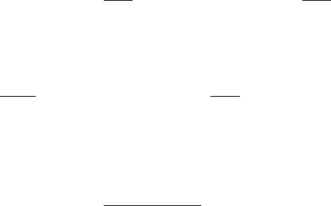
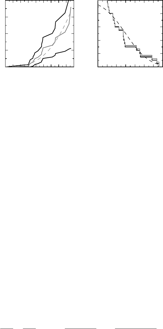
Example 11.6 Suppose that the logarithm of the sputum count in Section 6.2 instead describes

the survival time (in years) of 20 subjects after they have had a particular cancer diagnosis.

There are no censored data. Figure 11.7(a) shows the Nelson–Aalen estimate (solid gray

curve) of the true cumulative hazard (dashed curve) as well as pointwise conﬁdence limits

(solid black curves) for the (true) cumulative hazard. The jumps in 

(t) become larger as t

increases, for the obvious reason that the size of a jump is inversely proportional the number

at risk, of which there are fewer later than early on.

Figure 11.7(b) shows the true F

(t) (dashed line) as well as the two estimates of the

CDF discussed above, the Kaplan–Meier and Breslow respectively. We see that although

they are similar, they differ in details. In particular, we see that the Breslow estimator lies

above the Kaplan–Meier estimator everywhere. This is always true because of the inequality

−x

≥ 1 − x, which holds for all x, since it implies that

(t) =



s≤t

(1 − d

(s)) ≤



s≤t

−d

(s)

= e

−

(t)

310 HAZARDS AND CENSORED DATA

(a) (b)

Cumulative Hazard Λ(t)

9876543210

Time (months)

0.2

0.4

0.6

0.8

Survival function

(t)

98765432

Time (months)

Figure 11.7 (a) shows the cumulative hazard with conﬁdence limits (linearly interpolated),

with the true function as the dashed curve. (b) shows the true survival function (dashed)

together with the Kaplan–Meier estimate (black) and Breslow estimate (gray) thereof

(estimates as step functions).

In order to see where the Kaplan–Meier estimator comes from mathematically, we rewrite

the equation (11.1) as an integral equation in the survival function:

(t) = 1 +



(s−)d(−(s)). (11.5)

Its solution can be written as the ‘product integral’

(t) =



s≤t

(1 − d(s)),

a result due to the Swedish mathematician Ivar Fredholm in the early twentieth century (see

also Box 11.7). To obtain the Kaplan–Meier estimate of F (t) from this, we simply replace

d(t) with the Nelson–Aalen estimate d

(t) to get the expression

(t) =



s≤t

(1 − d

(s)).

In order to describe what knowledge we have obtained about F (t) from the Kaplan–Meier

estimator F

(t), we mostly rely on large-sample theory, and for this we need to compute

its variance. In the absence of censored data we know that F

(t) is the standard e-CDF, for

which the variance is F (t)F

(t)/n. The presence of censored data is expected to increase

this variance (compared with if the censored data were actually observed), because censoring

means an increase in uncertainty. We seek an expression for the variance V (F

(t)) in F

(t)

and d(t), and the trick for this is the observation that

F (t)

(t)

− 1 =



dF (s)

(s)F

(s−)



d(s)

(s−) −F (s)

THE KAPLAN–MEIER ESTIMATOR OF THE CDF 311

Box 11.7 The product-limit estimator

For a given function A(t), let the function B(t) satisfy the integral equation

B(t) = 1 +



B(s−)dA(s).

We can write B(t + h)asB(t) +



t+h

B(s−)dA(s) ≈ B(t)(1 + A(t)), which motivates

why, if A(t) is a step function, the solution of the integral equation is given by

B(t) =



s∈[0,t]

(1 + A(s)) = P

(A).

This deﬁnes the product-integral P

(A) for step functions, and by imitating how we de-

ﬁne the Stieltjes integral, this can be extended to many functions A(t) (those of bounded

variation). If A(t) is continuous we have that B(t) = e

A(t)

. (Note that A(t) and B(t) can

be matrix functions, which is useful in the study of Markov processes.) A consequence

of this is that the relation between (t) and F (t) deﬁned by equation 11.5 is that

(t) = P

(−), and that the Kaplan–Meier estimator is deﬁned by F

(t) = P

(−

The key result for product integration is Duhamel’s formula,

(A) − P

(B) =



s−

(A)(dA(s) −dB(s))P

(B).

Applied to A = 

and B = , it shows that

(t) − F

(t) =



(s−)(d

(s) −d(s))F

(t)/F

(s),

which can be rewritten as

(t) − F

(t)



(s−)

(s)

(d

(s) −d(s)) =



(s−)

(s)Y

(s)

dξ

(s). (11.6)

The compensator of this martingale is



(s−)

(1 − (s))d(s)

(s)

≈



(s)

(s)(Y

(s) −N

(s))

where ≈ means ‘can be estimated by’.

Estimating this integral in the obvious way, we ﬁnd that approximately

V (F

(t)) = F

(t)

(t),σ

(t) =



(s)

(s)(Y

(s) −N(s))

Martingale theory conﬁrms this (see Box 11.7). In the notation most often used, with d

the number of events at time t

, and r

as the number at risk at the same time, we have that

(t) =



≤t

− d

)

. (11.7)