Kelly J.J. Graduate Mathematical Physics, With MATHEMATICA Supplements
Подождите немного. Документ загружается.


26 1 Analytic Functions
is obtained using f z$z* f z f
'
z$z and gz $z*gzg
'
z$z for differentiable
functions and retaining only first-order terms,
lim
$z!0
f z $zgz $z f zgz
$z
lim
$z!0
f zg
'
z$z f
'
zgz$z
$z
(1.105)
such that
Fz f zgzF
'
z f zg
'
z f
'
zgz (1.106)
By similar reasoning one can verify all standard differentiation rules, subject to obvious
conditions on differentiability of the various parts. Perhaps the most important is the chain
rule
Fzg f z F
'
z
g
'
w f
'
z
w f z
(1.107)
provided that f is differentiable at z and that g is differentiable at w f z.
1.8 Properties of Analytic Functions
Suppose that f zux, yvx, y is analytic in domain D and suppose that the sec-
ond partial derivatives of the component functions u and v are continuous in D also. (We
will soon prove that analytic functions are infinitely differentiable so that the component
functions u and v must have continuous partial derivatives of all orders within D.) Differ-
entiation of the CR equations then gives
(u
(x
(v
(y
(
2
u
(x
2
(
2
v
(x(y
(
2
v
(y(x
(
2
u
(y
2
(
2
u
(x
2
(
2
u
(y
2
0 (1.108)
(v
(x
(u
(y
(
2
v
(x
2
(
2
u
(x(y
(
2
u
(y(x
(
2
v
(y
2
(
2
v
(x
2
(
2
v
(y
2
0 (1.109)
Therefore, both the real and imaginary components of f are harmonic functions that satisfy
Laplace’s equation. Furthermore, comparing the two-dimensional gradients
+u ˆx
(u
(x
ˆy
(u
(y
ˆx
(v
(y
ˆy
(v
(x
ˆn
+v (1.110)
+v ˆx
(v
(x
ˆy
(v
(y
ˆx
(u
(y
ˆy
(u
(x
ˆn
+u (1.111)
+u ,
+v 0 (1.112)
we find that lines of constant u (level curves) are orthogonal to lines of constant v anywhere
that f
'
z0. (Here ˆn represents the outward normal to the xy-plane.) If u represents a
potential function, then v represents the corresponding stream function (lines of force), or
vice versa.
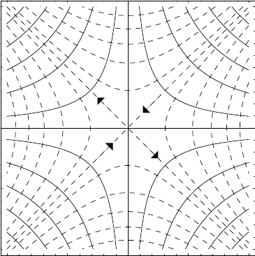
Consider, for example, f zz
2
with u x
2
y
2
and v 2xy. If we interpret v as an
electrostatic potential, then u represents lines of force. Figure 1.15 shows equipotentials
1.8 Properties of Analytic Functions 27
2 1 0 1 2
2
1
0
1
2
Figure 1.15. Level curves for f zz
2
u v are shown as solid for v anddashedforu.Ifthe
solid lines are interpreted as equipotentials, the dashed lines with directions given by
+v represent
lines of force.
as solid lines, positive in the first quadrant and alternating sign by quadrant, and lines of
force as dashed lines. The arrows indicate the direction of the force, as prescribed by
+v.
If electrodes were shaped with surfaces parallel to equipotentials, the interior field would
act as an electrostatic quadrupole lens, focussing a beam of positively-charged particles
along the 45° and 225° directions and defocussing along the 135° and 315° directions.
Alternatively, if v represents a magnetostatic potential, then u would represent magnetic
field lines. A beam of positively-charged particles moving into the page would be verti-
cally focussed and horizontally defocussed by a magnetic quadrupole lens whose iron pole
pieces have surfaces shaped by v - xy.
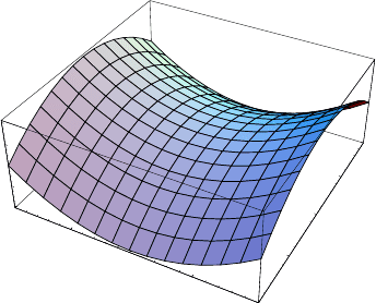
It is also easy to demonstrate that, although harmonic functions may have saddle
points, they cannot have extrema in the finite plane. Hence, neither component of an ana-
lytic function may have an extremum within the domain of analyticity. Figure 1.16 illus-
trates the typical saddle shape for components of an analytic function. Furthermore, the
average value of a harmonic function on a circle is equal to the value of that function of
the center of the circle. Proofs of these hopefully familiar properties of Laplace’s equation
are left to the exercises.
Suppose that Z
1
is a curve in the z-plane represented by the parametric equations z
1
t
x
1
t,y
1
t and that f z is analytic in a domain containing Z
1
, such that the image W
1
of
that curve in the w-plane is represented by w
1
t f z
1
t. The slopes of tangent lines at
a point z
0
and its image w
0
are related by the chain rule, such that
w
'
1
t f
'
zz
'
1
targ
w
'
1
t
arg
z
'
1
t
arg
f
'
z
0
(1.113)
28 1 Analytic Functions
2
1
0
1
2
2
1
0
1
2
4
2
0
2
4
2
1
0
1
Figure 1.16. Typical saddle: u x
2
y
2
.
Thus, the mapping f z rotates the tangent line through an angle arg f
'
z
0
. The tangent
to a second curve which passes through the same point z
0
is rotated by the same amount,
w
'
2
t f
'
zz
'
2
targ
w
'
2
t
arg
z
'
2
t
arg
f
'
z
0
(1.114)
such that angle between the two curves
argw
'
2
argw
'
1
argz
'
2
argz
'
1
(1.115)
is unchanged by the conformal transformation specified by an analytic function f z.Sim-
ilarly, distances in the immediate vicinity of z
0
are scaled by the factor f
'
z
0
, such that
w w
0
f
'
z
0
z z
0
(1.116)
Therefore, the image of a small triangle in the z-plane is a similar triangle in the w-plane
that is generally rotated and scaled in size.
1.9 Cauchy–Goursat Theorem
1.9.1 Simply Connected Regions
We have seen that the components of analytic functions are harmonic and might be stim-
ulated to pursue analogies with potential theory as far as possible. Remembering that the
line integral about a closed path vanishes for a potential derived from a conservative force,
we seek to evaluate
C
f zz
C
u x v y
C
u y v x (1.117)
for an analytic function f u v of z x y where ux, y and vx, y are real. If
we require Px, y and Qx, y to be differentiable within the simply connected region R
1.9 Cauchy–Goursat Theorem 29
enclosed by the simple closed contour C, we can apply Stoke’s theorem to prove
C
P x Q y
R
(Q
(x
(P
(y
x y (1.118)
Let
V P, Q, 0ˆn ,
+
V
(Q
(x
(P
(y
(1.119)
where ˆn is normal to the xy-plane and use
Λx, y, 0 as the line element and
Σ
ˆn x y as the area element to obtain
C
Λ,
V
R
Σ,
+
V
C
P x Q y
R
(Q
(x
(P
(y
x y (1.120)
Applying this result, known as Green’s theorem, to the real and imaginary parts of the line
integral separately, and using the CR conditions for analytic functions, we find
C
u x v y
R
(v
(x
(u
(y
x y 0 (1.121)
C
u y v x
R
(u
(x
(v
(y
x y 0 (1.122)
and conclude that
f analytic for z within C
C
f zz 0 (1.123)
This result was first obtained by Cauchy, but was later generalized by Goursat. The deriva-
tion above requires not only that f
'
z exist throughout R, but also that it be continuous
therein. The latter restriction can be removed.
Theorem 5. Cauchy–Goursat theorem: If a function f z is analytic at all points on and
within a simple closed contour C, then
C
f zz 0.
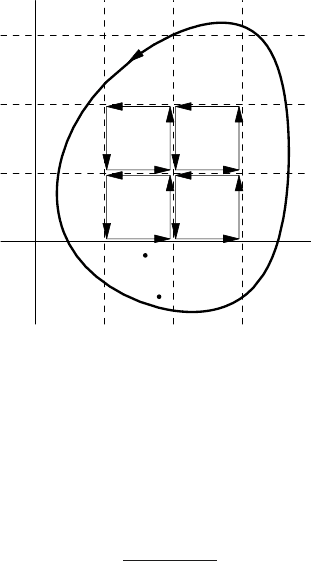
1.9.2 Proof
Consider the closed contour C sketched in Fig. 1.17. Divide the enclosed region R into a
grid of squares and partial squares, whereby
C
f zz
n
j1
C
j
f zz (1.124)
where the contributions made by shared interior boundaries cancel such that the net con-
tour integral is the sum of the exterior borders of outer partial squares. For each of these
cells, we construct the function
∆z, z
j
f z f z
j
z z
j
f
'
z
j
(1.125)
30 1 Analytic Functions
xRez
yImz
C
1
C
2
C
3
C
4
C
5
C
z
z
5
Figure 1.17. Proof of the Cauchy–Goursat theorem. Contours about four of the interior squares are
labeled C
14
.If f z is continuous, contributions to the contour integral from shared sides cancel,
leaving only the outer border C that passes through partial squares. In the partial square, labeled C
5
,
we identify two distinct points labeled z and z
5
.
where z and z
j
are distinct points within or on C
j
and evaluate its largest modulus
∆
j
Max
f z f z
j
z z
j
f
'
z
j
(1.126)
For any positive value of , a finite number of subdivisions is sufficient to ensure that all
∆
j
< because f z is differentiable. Thus, we can now write
f z f z
j
f
'
z
j
∆z, z
j
z z
j
(1.127)
for any z C
j
, such that
C
j
f zz f z
j
C
j
z f
'
z
j
C
j
z z
j
z
C
j
∆z, z
j
z z
j
z (1.128)
The first two terms obviously vanish, leaving
C
f zz
n
j1
C
j
∆z, z
j
z z
j
z (1.129)
which can be bounded by
C
f zz
n
j1
C
j
∆z, z
j
z z
j
z
(1.130)
1.9 Cauchy–Goursat Theorem 31
x
y
R
S
cccccc
4
C
1
C
2
C
3
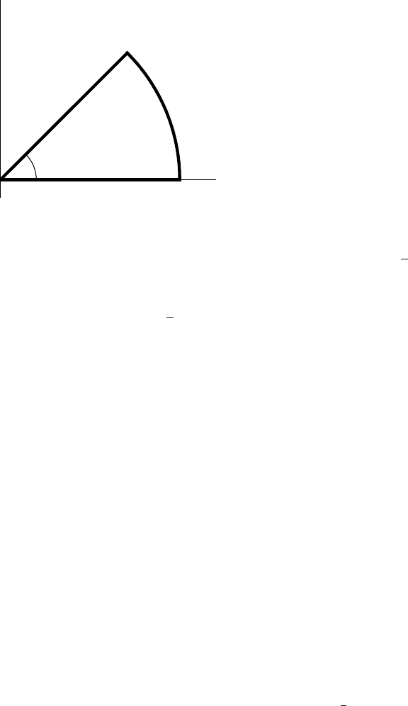
Figure 1.18. Wedge contour used for
0
Cosx
2
x.
If s
j
is the length of the longest side of partial square C
j
, then z z
j
2s
j
. Furthermore,
∆
j
< , such that
C
j
∆z, z
j
z z
j
z
2s
j
4s
j
L
j
(1.131)
where L
j
is the length of that part of C
j
that coincides with C. Because each factor is
bounded and ! 0 may be taken arbitrarily small, we find that
C
f zz is also arbitrar-
ily small and, hence, must vanish. Therefore, the Cauchy–Goursat theorem is established
without assuming that f
'
is continuous.
1.9.3 Example
Contour integration of analytic functions provides powerful new methods for evaluation
of otherwise intractable definite integrals. Although we will consider a wider variety later,
for now consider the integral
0
Cosx
2
x (1.132)
which arises in the Fresnel theory of diffraction. It appears to be difficult to evaluate this
integral using standard methods for real variables; nor is it obvious that this integral even
converges. On the other hand, the Cauchy–Goursat theorem ensures that
I
C
Expz
2
z 0 I
1
I
2
I
3
(1.133)
for a contour C consisting of a wedge of opening angle Θ
Π
4
closed by a circular arc at
R !; this contour is shown in Fig. 1.18. Consider first the circular arc where
z R
Θ
z
2
Exp
R
2
Cos2Θ
Exp
R
2
Sin2Θ
(1.134)
32 1 Analytic Functions
Recognizing that 0 < Sin2Θ < 1 is positive on the arc, the integrand is damped by a
factor of order
R
2
such that
R !I
2
0 I
1
I
3
(1.135)
where
I
1
0
Cosx
2
x
0
Sinx
2
x (1.136)
The return line is represented by
z
1
2
t z
1
2
t
z
2
t
2
(1.137)
such that
I
3
1
2
0
t
2
t
1
2
Π
2
(1.138)
Therefore, equating real and imaginary parts, we find
0
Cosx
2
x
0
Sinx
2
x
Π
8
(1.139)
rather easily. By representing the integrand in terms of analytic functions and choosing a
clever contour, one can perform a surprisingly diverse variety of integrals relatively pain-
lessly. In this case we even obtain two results for the price of one. (What a deal!)
1.10 Cauchy Integral Formula
1.10.1 Integration Around Nonanalytic Regions
Suppose that the region R R
1
R
2
enclosed by the simple closed contour C includes a
localized region R
2
where the function f is nonanalytic, but that f is analytic everywhere
else within C. The Cauchy–Goursat theorem can be applied to such a region by deforming
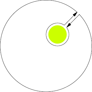
the contour in a manner that encapsulates the problematic region. Figure 1.19 illustrates
this technique. The colored region represents the nonanalytic region R
2
and the outer circle,
when closed, represents the contour C and is traversed in a positive, counterclockwise,
sense. Note that C need not actually be circular, but it is easier to draw that way. We
imagine drawing line A from C to a point just outside the nonanalytic region. The contour
C
2
goes around this region in a negative, clockwise sense, remaining within the analytic
region R
1
, ending close to its starting point. We then return along B to the contour C
1
.
The common path AB traversed in opposite directions between inner and outer contours
is sometimes called a contour wall and serves to create a simply connected region R
1
for
which the Cauchy–Goursat theorem requires
C
1
f zz
A
f zz
B
f zz
C
2
f zz 0 (1.140)
1.10 Cauchy Integral Formula 33
C
1
C
2
R
1
R
2
A
B
Figure 1.19. Construction of a contour wall and demonstration that a contour within an analytic
region may be shrink-wrapped around and enclosed nonanalytic region.
Recognizing that, for a continuous integrand, the contributions of A and B must become
equal and opposite as the separation between those paths becomes infinitesimal, we find
A
f zz
B
f zz 0
C
f zz
C
2
f zz (1.141)
Here the negative sign occurs because the inner contour is traversed in the opposite direc-
tion when reached by means of the contour wall. Therefore, the original contour can be
shrink-wrapped about the nonanalytic region without changing the value of the contour
integral.
If the path C encloses several localized nonanalytic regions, we simply construct sev-
eral contour walls. The net contour integral is then just the sum of the contributions
from shrink-wrapped contours around each nonanalytic region. Take care with the signs
though – if the original contour is traversed in a positive sense, the nonanalytic regions
are enclosed in a negative sense by the continuous deformed contour that circumvents
nonanalytic regions. However, recognizing that the entire contour integral vanishes and
that the contour walls cancel, the net integral for a simple contour that encloses nonan-
alytic regions reduces to the sum of the contributions made by shrink-wrapped contours
enclosing the nonanalytic regions in a positive sense. Therefore, if there are N isolated
nonanalytic regions within the simple closed contour C, we find
C
f zz
N
k1
C
k
f zz (1.142)
where each simple closed contour C
k
encloses one of the nonanalytic regions and is tra-
versed with the same sense as the original contour C.
We postpone consideration of extended nonanalytic regions to the next chapter, but in
the next few sections consider the important special case of an isolated singularity within
the contour.
34 1 Analytic Functions
1.10.2 Cauchy Integral Formula
Suppose that the contour C lies within a region R in which f z is analytic, but that it
surrounds another region R
'
in which f is not analytic. We demonstrated above that the
contour can be deformed, such that C ! C
'
where C
'
is immediately outside R
'
, without
changing the value of the contour integral
C
f zz
C
'
f zz (1.143)
Thus, a contour integral that encloses a single localized nonanalytic region can be shrink-
wrapped about the border of that region. This result is particularly useful for the case of
an isolated singularity for which the region of nonanalyticity consists of a single point z
0
.
Consider the integral
C
s
f s
s z
(1.144)
where f is analytic throughout the region enclosed by C while the integrand it singular
at z.Ifz is outside C the integral vanishes because the integrand is analytic at all points
within C. Alternatively, if z lies within C, we can reduce C to a small circle surrounding z,
such that
s z r
Θ
s r
Θ
Θ (1.145)
Thus, the integral can be approximated
C
s
f s
s z
* f z
C
r
Θ
Θ
r
Θ
2Π f z (1.146)
to arbitrary accuracy as r ! 0. Therefore, we obtain the Cauchy integral formula:
Theorem 6. Cauchy integral formula: If a function f z is analytic at all points on and
within a simple closed contour C, then f z
1
2Π
C
f s
sz
s for any interior point z.
This remarkably powerful theorem requires that the value of an analytic function at any
interior point is uniquely determined by its values on any surrounding closed curve and is
analogous to the two-dimensional form of Gauss’ theorem. The behavior of an analytic
function is severely constrained.
1.10.3 Example: Yukawa Field
Using elementary field theory, the virtual pion field surrounding a nucleon is represented
in momentum space by
˜
Φq
0
2
q
2
0
2
(1.147)
The spatial distribution is then obtained from the three-dimensional Fourier transform
Φr
3
q
2Π
3
q,r
˜
Φq
4Π
2Π
3
0
2
r
0
q Sinqr
q
2
0
2
q (1.148)
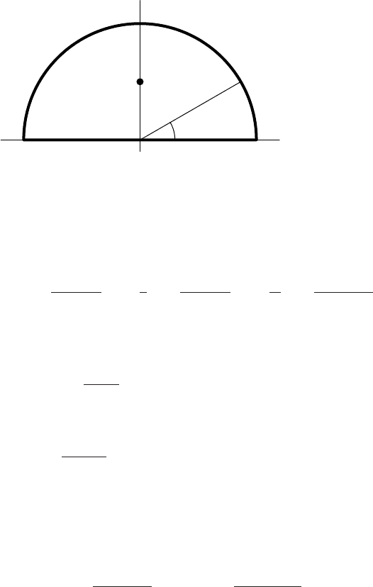
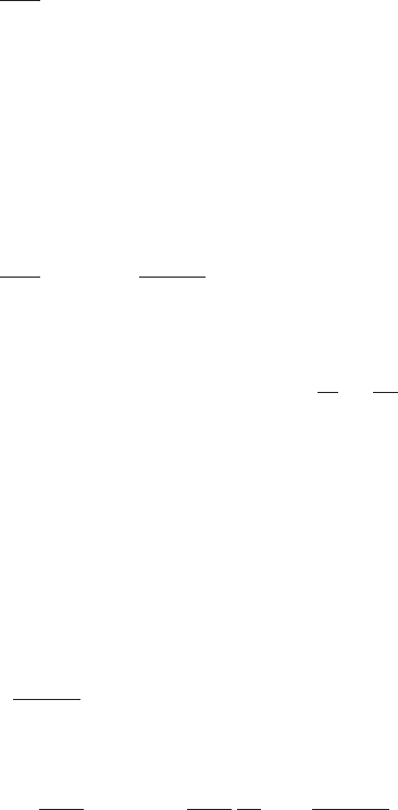
1.10 Cauchy Integral Formula 35
x
y
R
Θ
Figure 1.20. Great semicircle with enclosed pole at z 0.
where spherical symmetry and the multipole expansion of the plane wave have been used
to reduce the integral to one dimension. (Alternatively, the angular integrals can be evalu-
ated directly.) Recognizing that the integrand is even, we can write
0
q Sinqr
q
2
0
2
q
1
2
q Sinqr
q
2
0
2
q
1
2
q Expqr
q
2
0
2
q (1.149)
because the contribution from Cosqr vanishes by symmetry. Now consider the contour
integral
I0
C
gz
z 0
z (1.150)
where
gz
z
zr
z 0
(1.151)
is analytic in the upper half-plane.
If we choose a contour C, shown in Fig. 1.20, consisting of the real axis and a semicircle
in the upper half-plane with R !,affectionately called a great semicircle, this integral
can be expressed as
I0
q Expqr
q
2
0
2
q R
2
Π
0
Exp
rR
Θ
R
2
2Θ
0
2
Θ (1.152)
Using
Exp
rR
Θ
ExprR CosΘ ExprR SinΘ (1.153)
and recognizing that SinΘ > 0 in the upper half-plane, we realize that the contribution of
the circular arc decreases exponentially with R and vanishes in the limit R !. Therefore,
with the aid of the Cauchy integral formula
I0 2Πg0 Π
0r
(1.154)