Klipp E., Herwig R., Kowald A., Wierling C., Lehrach H. Systems Biology in Practice: Concepts, Implementation and Application
Подождите немного. Документ загружается.


ponents: the kernel that runs in the background performing the calculations and the
graphical user interface (GUI) that communicates with the kernel. The GUI has the
form of a so-called notebook that contains all the input, output, and graphics. Apart
from its numerical calculation and graphics abilities, Mathematica is renowned for
its capability to perform advanced symbolic calculations. Mathematica can be used
either by interactively invoking the available functions or by using the built-in pro-
gramming language to write larger routines and programs, which are also stored as
or within notebooks. For many specialized topics, Mathematica packages (a special
kind of notebook) that provide additional functionality are available. Two products
that ship with Mathematica, J/Link and MathLink, enable the two-way communica-
tion with Java or C/C++ code. This means that Mathematica can access external code
written in one of these languages and that the Mathematica kernel can actually be
called from other applications. The former is useful if an algorithm has already been
implemented in one of these languages or to speed up time-critical calculations that
would take too long if implemented in Mathematica itself. In the latter case other
programs can use the Mathematica kernel to perform high-level calculations or ren-
der graphics objects. Besides an excellent Help utility, there are also many sites on
the Internet that provide additional help and resources. The site http://mathworld.
wolfram.com contains a large repository of contributions from Mathematica users
all over the world. If a function or algorithm does not exist in Mathematica, it is
worthwhile to check this site before implementing it yourself. If questions and pro-
blems arise during the use of Mathematica, a valuable source of help is also the
newsgroup news://comp.soft-sys.math.mathematica.
The major rival of Mathematica is Matlab 6.5, produced by MathWorks (http://
www.mathworks.com). In many respects both products are very similar and it is up
to the taste of the user which one he prefers. Matlab is available for the same plat-
forms as Mathematica, has very strong numerical capabilities, and can also produce
many different forms of graphics. It also has its own programming language and
functions are stored in so-called M-files. Toolboxes (special M-files) add additional
functionality to the core Matlab distribution, and, like Mathematica, Matlab can be
called by external programs to perform high-level computations. A repository exists
for user-contributed files (http://www.mathworks.com/matlabcentral/fileexchange
and http://www.mathtools.net/MATLAB/toolboxes.html) as well as a newsgroup
(news://comp.soft-sys.matlab) for getting help. Despite these similarities, there are
also differences between the two programs. The table on the next page gives a very
short, superficial, and subjective list of important differences. The available space is
unfortunately not sufficient to go into more detail or describe finer differences.
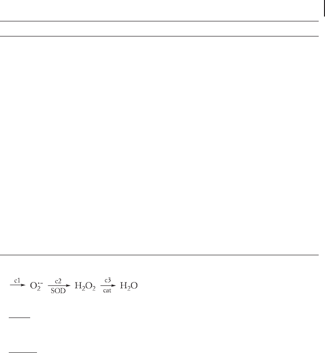
Let’s have a look at Mathematica and Matlab using a practical example. The super-
oxide radical, O
2
Q
–
, is a side product of the electron transport chain of mitochondria
and contributes to the oxidative stress a cell is exposed to. Different forms of the en-
zyme superoxide dismutase (SOD) exist that convert this harmful radical into hydro-
gen peroxide, H
2
O
2
. This itself causes oxidative stress, and again different enzymes,
such as catalase (cat) or glutathione peroxidase, exist to convert it into water. If we
want to describe this system, we can write down the following reaction scheme and
set of differential equations.
420
14 Modeling Tools
dO
2
Q
dt
c
1
c
2
SOD O
2
Q
dH
2
O
2
dt
c
2
SOD O
2
Q
c
3
cat H
2
O
2
14.1.1.1 Mathematica Example
First we define the differential equations (and assign them to the variables eq1 and
eq2) and specify the numerical values for the constants.
eq1 = O2'[t] == c1-c2*SOD*O2[t];
eq2 = H2O2'[t] == c2*SOD*O2[t]-c3*cat*H2O2[t];
par = {c1?6.6*10
–7
,c2?1.6*10
9
,c3?3.4*10
7
, SOD?10
–5
, cat?10
–5
}
Now we can solve the equations numerically with the function NDSolve and as-
sign the result to the variable “sol.” As boundary conditions we specify that the initial
concentrations of superoxide and hydrogen peroxide are zero and instruct NDSolve
to find a solution for the first 0.01 seconds. NDSolve returns an interpolating func-
tion object, which can be used to obtain numerical values of the solution for any
time point between 0 and 0.01. We see that at 0.01 seconds the concentrations are in
421
14.1 Modeling and Visualization
Topic Mathematica Matlab
Debugging Cumbersome and difficult. No de-
dicated debugging facility.
Dedicated debugger allows one to
single-step through M-files using break-
points.
Add-ons Many standard packages ship with
Mathematica and are included in
the price.
Many important toolboxes have to be
bought separately. See http://
www.mathworks.com/products/
product_listing.
Deployment User needs Mathematica to per-
form the calculations specified in
notebooks.
Separately available compiler allows one
to produce standalone applications.
Symbolic compu-
tation
Excellent built-in capabilities. Possible with commercial toolbox.
Storage All input, output, and graphics are
stored in a single notebook.
Functions are stored in individual
M-files. A large project can have hun-
dreds of M-files.
Graphics Graphics are embedded in a note-
book and cannot be changed after
their creation.
Graphics appear in a separate window
and can be manipulated as long as the
window exists.
ODE model
building
Differential equations are specified
explicitly.
Dynamical processes can be graphically
constructed with Simulink, a compa-
nion product of Matlab.

the nanomolar range and the level of H
2
O
2
is approximately 50-fold higher than the
concentration of superoxide. Finally, we use Plot to produce a graphic showing the
time course of the variable concentrations. We specify several options such as axes la-
bels and colors to make the plot more informative.
sol = NDSolve[{eq1, eq2, O2[0]==0, H2O2[0]==0}/.par, {O2, H2O2}, {t,0,0.01}]
{O2[0.01], H2O2[0.01]}/.sol ⇒ {{4.125*10
–11
, 1.84552*10
–9
}}
Plot[Evaluate[{O2[t], H2O2[t]/50}/.sol], {t,0,0.01}, PlotRange->All,
PlotStyle->{Hue[0.9],Hue[0.6]}, AxesLabel->{“time”,“concentration”}];
14.1.1.2 Matlab Example
In Matlab the routine that solves the ODE systems requires as one of its arguments
a function that evaluates the right-hand side of the ODE system for given times and
variable values. Because the example system is so small, we can define this function
as an inline function and avoid writing a separate M-file. Next the options for the
ODE solver are defined. The absolute values of the solution are very small, and there-
fore the absolute tolerance has to be adjusted accordingly.
dydt = inline(‘[c1-c2*SOD*y(1);c2*SOD*y(1)-c3*cat*y(2)]‘,’t‘,’y‘,’tmp‘,’
SOD‘,’cat‘,’c1‘,’c2‘,’c3’);
options = odeset(‘OutputFcn’,[ ], ‘AbsTol’, 1e-30, ‘RelTol’, 1e-6);
Now ode45 is called, which solves the ODE system for the specified time span. In
addition to dydt, which evaluates the derivatives,we also supply the starting concentra-
tions of the variables and the numerical values for the constants that were used in
dydt. ode45 is only one of a whole set (ode45, ode23, ode113, ode15s, ode23s, ode23t,
and ode23tb) of possible solvers with different properties (differing in accuracy or suit-
ability for stiff problems). The function returns a vector, t, holding time points for
which a solution is returned and a matrix, y, that contains the variable values at these
time points. To find out which concentration exists at a given time, the function “in-
terp1” can be used, which also interpolates between existing time points if necessary.
Finally, the resulting time course is plotted and the axes are labeled appropriately.
[t, y] = ode45(dydt, [0,0.01], [0;0], options, 1e-5, 1e-5, 6.6e-7, 1.6e9, 3.4e7);
interp1(t,y,0.01) ⇒ 4.125*10
–11
, 1.84552*10
–9
plot(t, y(:,1), t, y(:,2)/50)
xlabel(‘time’)
ylabel(‘concentration’)
14.1.2
Gepasi
Matlab and Mathematica are huge and expensive general-purpose tools for mathe-
matical modeling. They can be used to model anything that can be modeled, but at
the cost of a steep learning curve. The opposite approach is used by specialized tools
422
14 Modeling Tools
that are designed for a certain task. Gepasi is one of these tools that have been devel-
oped for the modeling of biochemical reaction systems. It was written by Pedro
Mendes (Mendes 1993, 1997) and is available free of charge (http://www.gepasi.org).
It runs native under Microsoft Windows but can also be used under Unix/Linux in
connection with the Wine emulator (http://www.winehq.com).
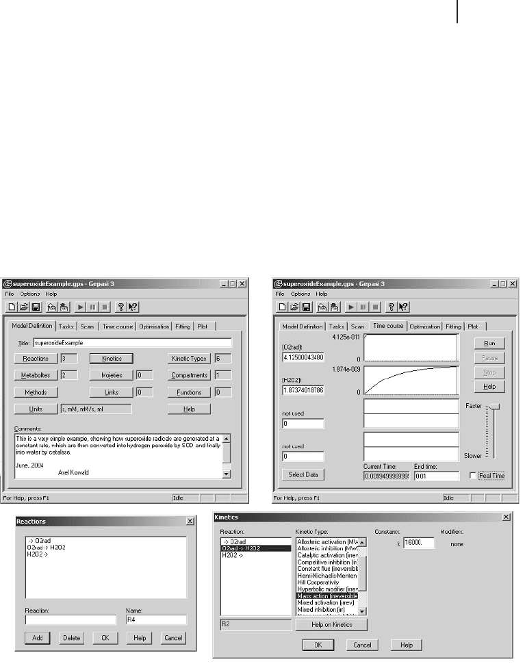
In Gepasi, reactions are entered not as differential equations but rather in a nota-
tion similar to chemical reactions (Fig. 14.1). Each reaction has to be assigned to a
specific kinetics, and Gepasi allows the user to select from a large range of prede-
fined kinetics types (Michaelis-Menten, Hill Kinetics, Uni-Uni, etc.). In addition it is
also possible to create user-defined kinetics types. Once a system is defined, the pro-
gram allows one to perform several tasks such as plotting a time course, scanning
the parameter space, fitting models to data, optimizing any function of the model,
and performing metabolic control analysis and linear stability analysis.
423
14.1 Modeling and Visualization
Fig. 14.1 The simulation tool Gepasi. Top left:
The main window, which contains tabs for activ-
ities such as input of the reaction system, calcu-
lating a time course, fitting the system to experi-
mental data or scanning the parameter space.
Bottom left: Reactions are entered in a chemical
notation, not as ODEs. Irreversible reactions are
entered with the symbol -> and reversible reac-
tions with an equal sign (=). Bottom right:
A kinetics has to be assigned to each reaction
and the necessary numerical constants have to
be specified. Top right: If the system has been
defined, Gepasi can calculate the time course
of selected variables.

It is also possible to create multi-compartment models with Gepasi to model reac-
tions that take place, for instance, in the cytoplasm and the nucleus. If a metabolite
crosses a boundary between two compartments of different volume, the change of
concentration in the originating compartment is not equal to that in the destination
compartment. Gepasi automatically takes care of the conversions between concentra-
tions into absolute amounts and back, which is necessary for the calculations. Apart
from its own format, Gepasi can also save and load models that are described in the
Systems Biology Markup Language (SBML) level 1 (see Section 14.2.2).
Gepasi is a handy tool that is designed to perform many of the standard tasks for
studying a system of biochemical reactions. It is easy to handle, except that one has
to get used to the strange fact that all windows are of a fixed size and rather small.
Graphical simulation results, however, can also be redirected to a companion pro-
gram, gnuplot, which does not have these restrictions.
14.1.3
E-Cell
The E-Cell system, initially developed in 1996 at Keio University (Japan), is designed
for the simulation of cellular processes. Its first version (E-Cell 1) was used for the
construction of a hypothetical cell model with 127 genes, which proved to be suffi-
cient for the modeling of transcription, translation, energy production, and phospho-
lipid synthesis. For this model, a gene collection of Mycoplasma genitalium was em-
ployed as template (Tomita et al. 1999), as this microorganism is equipped with one
of the smallest genomes known. A further model developed for use with E-Cell deals
with the mitochondrial metabolism and describes several pathways and processes
such as the respiratory chain, the TCA cycle, the fatty acid b-oxidation, and the meta-
bolite transport system (Yugi and Tomita 2004).
The latest version of E-Cell (E-Cell 3, http://www.e-cell.org/) – as well as E-Cell 2 –
runs under Microsoft Windows and Linux. E-Cell 3 allows the user to perform multi-
algorithm calculations, e.g., deterministic models described by ODEs can coexist
with stochastic models. Since different cellular processes take place on different
timescales – e.g., enzymatic reactions occur on the order of milliseconds and gene
regulatory events happen on the order of minutes or hours – E-Cell 3 also includes
an algorithm that handles the multiple timescales associated with different cellular
processes (Takahashi et al. 2004).
E-Cell models are constructed by employing three fundamental object classes:
substance, reactor, and system. Substances represent state variables. Reactors are
processes that operate on the state variables. Systems can contain other objects and
represent logical and/or physical compartments that can be used for the develop-
ment of hierarchical models for cellular systems.
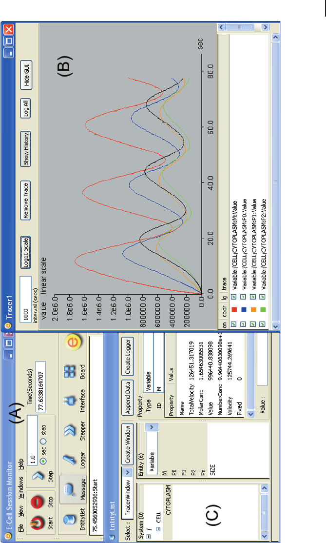
Figure 14.2a shows the Session Monitor of E-Cell. Via the Session Monitor, simu-
lations of previously loaded models can be performed. Simulation results can be
plotted in a diagram using the TracerWindow (Fig. 14.2 b), which is created via the
EntityList window. The EntityList window (Fig. 14.2 c) further presents the model
hierarchy given by the nested structure of systems and a list of the variables (or pro-
424
14 Modeling Tools
425
14.1 Modeling and Visualization
Fig. 14.2 The E-Cell system. (a) The Session Monitor is used to load models and perform simu-
lations. Simulation results can be viewed, e.g., via the TracerWindow (b). The EntityList (c) offers
functionalities to browse the model or to edit properties of the variables and processes.

cesses) contained in the selected system. Furthermore, it is used to edit variable or
process properties such as the values of the initial concentrations or kinetic con-
stants.
A model file (with the file extension *.eml) can be created either from a separate
script file (with the file extension *.em) or directly via a separate application, the
Model Editor. In addition to this a further system called GEM (Genome-based E-Cell
Modeling) has been developed. The purpose of this system is to automate the gen-
eration of E-Cell models. GEM implements a powerful annotation system that uti-
lizes public databases. Via GEM, E-Cell models can be generated simply from gen-
ome sequences (Ishii et al. 2004).
14.1.4
PyBioS
PyBioS is designed for applications in systems biology and supports modeling and
simulation. In contrast to e.g., Gepasi or E-Cell, which are installed locally, PyBioS is
a Web-based environment running on a server that is accessible via http://pybios.
molgen.mpg.de/. The purpose of PyBioS is to provide a framework for the conduc-
tion of kinetic models of various sizes and levels of granularity. The tool can be used
as a standalone modeling platform for ediding and analyzing biochemical models in
order to predict the time-dependent behavior of the models. Alternatively, the plat-
form offers the possibility of database interfaces (e.g., KEGG, Reactome) where
models can automatically be populated from database information. In particular, the
high level of automation enables the analysis of large models.
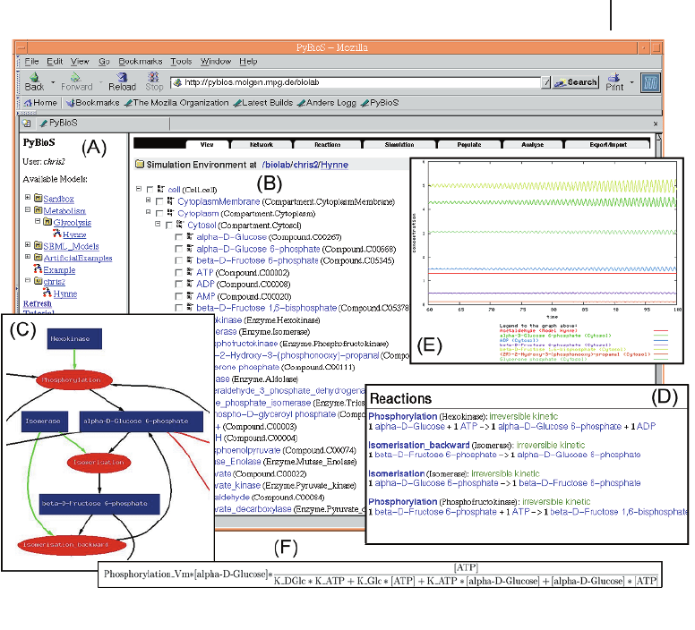
Figure 14.3 shows screenshots of the PyBioS modeling and simulation environ-
ment. Predefined models can be selected from a model repository. Alternatively,
users can also create their own models. Using the “View” tab, the user can inspect
the hierarchical model. A list of all reactions of the model and a diagram of the
whole reaction network are available via the “Reactions” and “Network” tabs, respec-
tively. Model simulations performed by numerical integration of ordinary differential
equation systems (ODEs) are possible via the “Simulation” tab. The “Population” tab
offers functions for the creation and modification of a model, e.g., forms to edit ki-
netic parameters and initial concentrations of model components representing state
variables. One question a systems biologist might be interested in is how the steady-
state behavior of a system might change if one parameter (e.g., the rate of glucose
uptake of a cell) is varied. PyBioS provides functionalities to scan the steady-state be-
havior (via successive simulations or root finding) given a varying parameter. This
function, which also includes basic stability analysis, as well as other functions such
as the computation of conservation relations are provided via the “Analysis” tab. Fi-
nally, via the “Export/Import” tab users can exchange models with other modeling
systems, e.g., via SBML language Level 1 (see Section 14.2.2). One important feature
of PyBioS is the possibility of using information of public databases directly for the
creation of models. It offers, e.g., an interface to the metabolic data of KEGG (see
Section 13.2) or an interface to the Reactome database (see Section 13.7), the latter
still being under development.
426
14 Modeling Tools
The underlying object-oriented structure of PyBioS entails a set of predefined ob-
ject classes for biological entities (in the following, referred to as BioObjects). Avail-
able BioObjects are Cell, Compartment, Compound, Chromosome, Polypeptide, Pro-
tein, Enzyme, Complex, Gene, etc. All of these BioObjects correspond to their re-
spective biological counterpart and can be used for the creation of computational
models that are hierarchically ordered according to fundamental cytological, and mo-
lecular structures (e. g., compartments or molecule complexes). Object-specific infor-
mation is stored as properties of the BioObjects; for instance, each BioObject has an
identifier and a concentration, and a Chromosome or Polypeptide can have a nucleo-
427
14.1 Modeling and Visualization
Fig. 14.3 The PyBioS simulation environment.
A particular model can be selected from the
model repository (a) and its hierarchical model
structure can be inspected via the “View” tab at
the top of the browser window (b). A graphical
representation of the model is provided by an
automatically generated network diagram (ac-
cessible via the “Network” tab), e.g., (c) shows
the forward and reverse reaction of the isomeri-
zation of glucose-phosphate to fructose-phos-
phate of a glycolysis model. The “Reactions” tab
offers an overview of all reactions of the model
(d). Simulations can be performed via the “Si-
mulation” tab (e). A simulation is based on an
automatically generated mathematical model
derived from the corresponding object-oriented
model that comprises the network of all reac-
tions and their respective kinetics (f).

tide or amino acid sequence, respectively. Furthermore, each BioObject can have one
or more actions. For example, an action can be a chemical reaction or a transport
process of molecules between different compartments. Actions describe the stoichio-
metry of the reactions and their kinetics. PyBioS provides a list of several predefined
kinetic laws from which an appropriate one can be chosen for a specific reaction.
Moreover, users can define their own kinetic laws. The hierarchical object-oriented
model composed of several BioObjects is internally stored in an object-oriented data-
base and is used for further applications provided by PyBioS. For instance, for a time
course simulation, the object-oriented model is used for the automatic generation of
a system of ODEs.
14.1.5
Systems Biology Workbench
So far we have discussed quite a few different modeling tools, and more will be de-
scribed in the next sections. One reason for this multitude of simulation tools is that
no single tool can provide all the possible simulation methods and ideas that are
available. This is especially true since new experimental techniques and theoretical
insights constantly stimulate the development of new ways to simulate and analyze
biological systems. Consequently, different researchers have written different tools
in different languages running on different platforms. A serious problem with this
development is that most tools save models in their own format, which is not compa-
tible with the other tools. Accordingly, models cannot easily be exchanged between
tools but have to be re-implemented by hand. Another problem is the overhead in-
volved with programming parts of the tool that are not part of the actual core func-
tion. This means that although a program might be specialized in analyzing the to-
pology of a reaction network, it also has to provide means for the input and output of
the reaction details.
Two closely related projects aim at tackling these problems. One is the develop-
ment of a common format for describing models. This resulted in the development
of the Systems Biology Markup Language (SBML), which is described in detail in
Section 14.2.2. The other project is the Systems Biology Workbench (SBW) (Hucka
et al. 2002), which is a software system that enables different tools to communicate
with each other (http://www.sys-bio.org). Thus, SBW-enabled tools can use services
provided by other modules and in turn advertise their own specialized services. Fig-
ure 14.4 gives an overview of SBW and some of the currently available SBW-enabled
programs. At the center of the system is the SBW broker that receives messages
from one module and relays them to other modules. Let’s have a quick look at this
mechanism using JDesigner and Jarnac, two modules that come with the SBW stan-
dard installation. JDesigner is a program for the graphical creation of reaction net-
works, and Jarnac is a tool for the numerical simulation of such networks (time
course and steady state). Jarnac runs in the background and advertises its services to
the SBW broker. JDesigner contacts the broker to find out which services are avail-
able and displays the found services in a special pull-down menu called SBW. A reac-
tion model that has been created in JDesigner can now be sent to the simulation ser-
428
14 Modeling Tools
vice of Jarnac. A dialog box opens to enter the necessary details for the simulation,
and then the broker calls the simulation service of Jarnac. After a time course simu-
lation finishes, the result is transmitted back to JDesigner (via the broker) and can
be displayed. Further technical details of the SBW system are given in Sauro et al.
(2003).
The representative list of SBW-enabled programs shown in Fig. 14.4 contains pro-
grams specialized in the graphical creation of reaction networks (JDesigner and Cell-
Designer), simulation tools (Jarnac and TauLeapService), analysis and optimization
tools (Metatool, Bifurcation and Optimization), and utilities such as the Inspector
module, which provides information about other modules.
SBW and SBML are very interesting developments that hopefully will help to facil-
itate the exchange of biological models and thus stimulate the discussion and coop-
eration among modelers. The more tool-writers adopt the SBML format and render
their applications SBW aware, the more powerful this approach will be. Steps are un-
der way to integrate BioSPICE (http://www.biospice.org) into the SBW framework
(Sauro et al. 2003), which will strengthen SBW’s data handling capabilities and sup-
port its status as the de facto standard for modeling in systems biology. To give read-
ers an idea of what working with SBW is like, we will now describe the programs
JDesigner and CellDesigner in more detail.
14.1.5.1 JDesigner
JDesigner is a Microsoft Windows program that is included with the SBW installa-
tion. It can be used in combination with SBW or as standalone application. If used
alone, it is a graphical network designer. In this mode only the graphics canvas,
which can be seen in the top right part of Fig. 14.5, is available. An icon bar allows
the easy construction of networks consisting of compartments, molecular species,
and reactions between the species. In the example shown, the network consists of
429
14.1 Modeling and Visualization
SBW
JDesigner
Jarnac
CellDesigner
Optimization
Bifurcation
Inspector
Metatool
TauLeapService
Fig. 14.4 The systems biology workbench
(SBW) and SBW-enabled programs. The SBW
broker module (in the center) forms the heart of
the SBW and provides message passing and re-
mote procedure invocation for SBW-enabled
programs. The programs can concentrate on a
specialized task such as graphical model build-
ing (JDesigner, CellDesigner) or simulation and
analysis (Jarnac, TauLeapService, Metatool, Opti-
mization, Bifurcation) and otherwise use the
capabilities of already-existing modules.