Lehner G. Electromagnetic Field Theory for Engineers and Physicists

Подождите немного. Документ загружается.

244 The Stationary Current Density Field

Notice that this formula is a complete analogue to Sect. 2.11.2. We therefore find

by just replacing by

(4.50)

, (4.51)

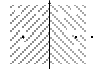
The current density fields correspond to the figures of the electric field of Sect.

2.11.2. Two limits are most important. For an insulator in region 2 we have:

This case is illustrated in Fig. 4.13. Conversely, Fig. 4.14 shows the case when

region 2 is filled with a perfect conductor. results in

Fig. 4.13 represents a Neumann boundary condition and Fig. 4.14 the

Dirichlet boundary condition

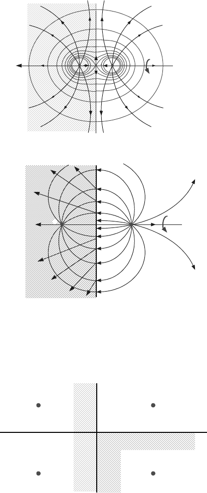
Using these results allows to solve an abundance of problems by

superposition of appropriate sources. For instance, Fig. 4.15 suggests how to solve

the problem of a point source in a quadrant where the boundary on one side

consists of a perfect conductor, while the other side borders a perfect insulator.

Conversely, if both media are perfect conductors, then Fig. 4.16 suggests a solution

path.

By taking a limit one may transition to a dipole source and, for instance, solve

the problem of a sphere embedded in some uniform medium of different

conductivity, by superposition of dipole current density and uniform current

density (this is analog to Section 2.12).

Fig. 4.12

-a a

I ’ I I ’’

εκ

I' I

–

------------------

I'' I

2κ

------------------

κ 0=

I' I=

I'' 0=







∞→

I' I–=

I'' 0=







∂ϕ ∂n⁄ 0=

ϕ const.=

4.5 Some Current Density Fields 245

Fig. 4.13

Fig. 4.14

Fig. 4.15

κ finite

κ 0=

κ∞→

-I

246 The Stationary Current Density Field

4.5.2 Line Sources

Basically, all that was said for line charges applies to line sources as well. If r is the

perpendicular distance to a uniform line source in the infinite space, then

(4.52)

, (4.53)

and

(4.54)

Fig. 4.16

κ finite

κ∞→

-I

Fig. 4.17

κ finite

κ 0=

κ∞→

-–

Il⁄

2πlr

-----------=

2πκlr

---------------=

ϕ r()

2πκl

------------

-----ln–=

4.5 Some Current Density Fields 247

Furthermore, we may apply all examples of Section 4.5.1 to line sources by

substituting I by I/l in Figs. 4.12 through 4.16. This also holds for the two eqs.

(4.50) and (4.51).

The solutions resulting thereof can be used as a starting point to solve

additional plane problems by conformal mapping. For instance, the field shown in

Fig. 4.18 results from Fig. 4.17 by the conformal mapping (similar to

Example 6 of Sect. 3.12).

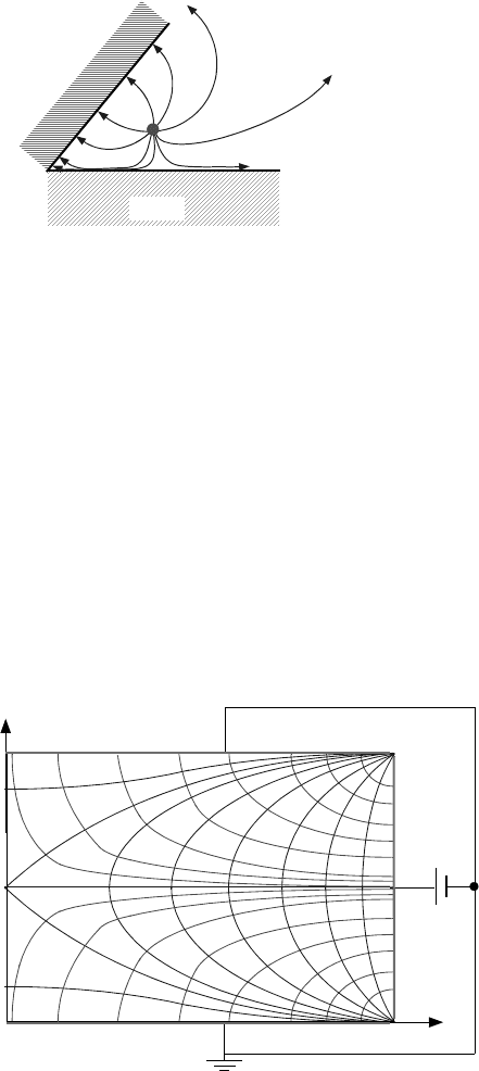
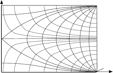
4.5.3 Mixed Boundary Value Problem

To demonstrate the separation of variable method, we choose for simplicity reasons

a plane and, mixed boundary value problem for Laplace’s equation .

Consider the rectangular piece of a uniform conductor with the sides a and b where

a voltage is applied as shown in Fig. 4.19. The two sides and are

coated with a very good conductor (like silver) and are grounded. The side

ξ z

Fig. 4.18

κ 0=

κ∞→

κ finite

∇

ϕ 0=

Fig. 4.19

ϕϕ

ϕ 0=

xa=

y = b

y 0= yb=

xa=

248 The Stationary Current Density Field

shall also be coated with silver but the potential there shall be . There is no

conducting material at the side and therefore, the current density lines have

to be parallel to that boundary, which means that . We summarize the

boundary conditions:

(4.55)

In order to meet the boundary conditions for y, the y-dependent part is written as

This determines the form of the x-dependency, since the problem is independent of

One needs to let in order to satisfy the condition for . For

, this results in the requirement

i.e.,

Furthermore, letting , satisfies for . Then

(4.56)

There is potentially an additional term stemming from the case

. However, it vanishes because of the boundary conditions. Obviously

eq. (4.56) satisfies all boundary conditions, except that at . This needs to be

taken care of. One has to find the coefficients in such a way that

(4.57)

Using the usual trick, one multiplies this equation by and integrates y

from 0 to b:

ϕϕ

x 0=

∂ϕ dn⁄ 0=

ϕ 0= for

y 0=

yb=







ϕϕ

= for xa=

n∂

∂ϕ

x∂

∂ϕ

0== for x 0=











Aky()cos Bky()sin+

Ckx()cosh Dkx()sinh+

A 0= ϕ 0= y 0=

yb=

kb()sin 0=

kb nπ=

nπ

------==

D 0= ∂ϕ dn⁄ 0= x 0=

ϕ xy,() C

nπx

---------





cosh

nπy

---------





sin

n 1=

∞

∑

ABy+()CDx+()

k 0=

xa=

nπa

----------





cosh

nπy

---------





sin

n 1=

∞

∑

n'πyb⁄()sin

4.5 Some Current Density Fields 249

With the orthogonality relation (3.76) one obtains

Integrating the right side gives

This makes

(4.58)

i.e.,

(4.59)

and with (4.56), the solution is finally

(4.60)

The problem may also be interpreted as a boundary value problem for , because

(4.61)

applies to as well. However the boundary conditions are different from those for

in (4.55). Now one has the situation as illustrated in Fig. 4.20.

(4.62)

n'πy

----------





sin yd

∫

nπa

----------





cosh

nπy

---------





sin

n'πy

----------





sin yd

∫

n 1=

∞

∑

---

n'πa

-----------





cosh ϕ

n'πy

----------





sin yd

∫

n'πy

----------





sin yd

∫

n'π

-------

0cos n'π()cos–[]

n'π

-------

11–()

–[]==

2ϕ

nπ

nπa

----------





cosh

----------------------------------

11–()

–[]=

4ϕ

nπ

nπa

----------





cosh

----------------------------------

for n 135…,,=

0 for n 246…,,=











4ϕ

---------

2n 1+

---------------

2n 1+()πx

---------------------------





cosh

2n 1+()πa

---------------------------





cosh

---------------------------------------------

2n 1+()πy

---------------------------





sin

n 0=

∞

∑

∇

ψ 0=

y∂

∂ψ

–0= = for

y 0=

yb=

x 0=











x∂

∂ψ

2ϕ

δ yb–()δy()–[]= = for xa=











250 The Stationary Current Density Field

The factor in front of the δ-function is due to the behavior of the potential

along . If we view this potential as a function of y, then

This implies that there is a discontinuity by at both locations, and

The Ansatz

(4.63)

satisfies the first three conditions of eq. (4.62), but not the last one. This requires

from which one gets

(4.64)

And finally

(4.65)

The two results (4.60) and (4.65) are equivalent, and enable one to find the field.

Both and have to satisfy the Cauchy-Riemann condition:

Fig. 4.20

yb=

∞=

∞–=

xa=

2ϕ

xa=

ϕ ay,() ϕ

= for 0 yb<<

ϕ ay,() ϕ

–=for by2b<< by0 .<<–,

2ϕ

y 0=

yb=

ψ xy,() d

nπx

---------





sinh

nπy

---------





cos

n 1=

∞

∑

nπ

------

nπa

----------





cosh

nπy

---------





cos

n 1=

∞

∑

2ϕ

δ yb–()δy()–[]=

2ϕ

nπ

nπa

----------





cosh

----------------------------------

1–()

1–[]=

ψ xy,()

4ϕ

---------–

2n 1+

---------------

2n 1+()πx

---------------------------





sinh

2n 1+()πa

---------------------------





cosh

---------------------------------------------

2n 1+()πy

---------------------------





cos

n 0=

∞

∑

ϕψ

4.5 Some Current Density Fields 251

which is the case. Of course, one could have used this relation to calculate ,

which would have been easier than solving the boundary value problem again.

Knowing and allows to write the complex potential of the field:

Because of

we re-write w(z)

which gives

(4.66)

This represents the conformal mapping which solves this particular problem.

The current density function allows to calculate the resistance of the setup or

rather its inverse the conductance:

If d represents the thickness of a conductive layer, it is then

x∂

∂ϕ

y∂

∂ψ

y∂

∂ϕ

x∂

∂ψ

,–=

ϕψ

wz() ϕxy,()iψ xy,()+=

z()sinh xiy+()sinh x()sinh iy()cosh x()cosh iy()sinh+==

x()sinh y()cos ix()cosh y()sin+=

wz()

4ϕ

---------

⋅=

2n 1+()πx

---------------------------cosh

2n 1+()πy

---------------------------sin i

2n 1+()πx

---------------------------sinh

2n 1+()πy

---------------------------cos–

2n 1+()

2n 1+()πa

---------------------------





cosh

--------------------------------------------------------------------------------------------------------------------------------------------------------------

n 0=

∞

∑

⋅

wz()

4ϕ

-----------

2n 1+()πz

--------------------------sinh

2n 1+()

2n 1+()πa

---------------------------





cosh

------------------------------------------------------------------

n 0=

∞

∑

–=

---

0–

---------------===

Idg

a 0,()

()

∫

κ dE

a 0,()

()

∫

κ– d

y∂

∂ψ

a 0,()

()

∫

κ– d ψd

a 0,()

()

∫

κ– d ψ ab,()ψa 0,()–[]

252 The Stationary Current Density Field

And then for the conductance

(4.67)

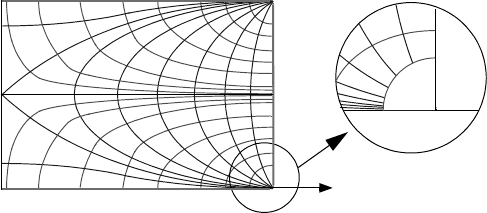
The Conductance becomes infinitely large, which is a consequence of the idealized

assumptions. The potential is discontinuous at the corners , and

, respectively. This is the reason why there, the electric field is infinitely

large, as we have seen from the boundary conditions (4.62). Furthermore, the

current density, and even the integrated total current becomes infinite, i.e.,

and are not finite. The singularity can be eliminated if we remove small

pieces from the corners, while following a current density line (Fig. 4.21).

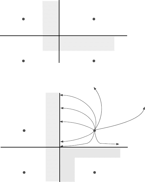
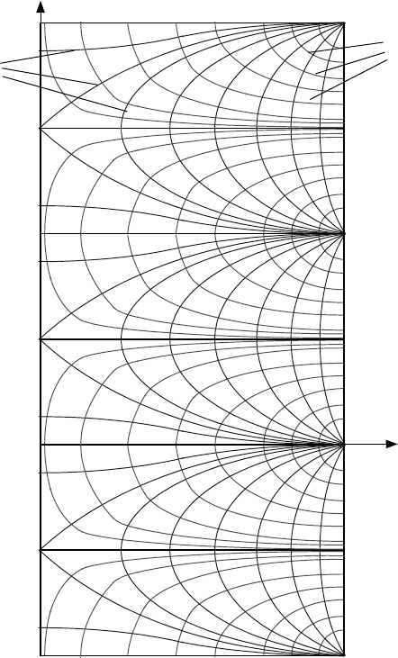
Notice that in solving this problem, one may consider a number of other

problems as well.Fig. 4.22 shows a larger picture of the field. Fig. 4.22 allows a

number of different interpretations. For instance, one may pick the range from

through as shown in Fig. 4.23 and regard it as the solution

of a different boundary value problem. Fig. 4.24 shows the solution when taking

only the range form 0 through b/2. Furthermore, one can find a new meaning by

exchanging the roles of and . For instance, this transforms Fig. 4.23 into a

point like current source, injected at and , while the current is

drained off on the three sides and , while the side with

borders an insulator (disregarding the point like source), illustrated in Fig. 4.25.

Calculating the resistance in this case, one finds that it diverges. The reason is the

singularity of the current injection at and . We have discussed this

situation already in conjunction with the diverging conductance of eq. (4.67). In the

present interpretation, the current remains finite, while the quantity which we

interpret as being the potential diverges. Finite current when voltage is

infinite means that resistance has to be infinite. As before, this divergence is of

4κϕ

----------------

2n 1+

---------------

2n 1+()πa

---------------------------tanh

n 0=

∞

∑

8κd

----------

2n 1+()πa

---------------------------tanh

2n 1+()

---------------------------------------

∞⇒

n 0=

∞

∑

xa= y 0=

yb=

ψ ab,()

ψ a 0,()

Fig. 4.21

ϕϕ

ϕ 0=

ψ const=

yb2⁄–= y +b 2⁄=

ϕψ

xa= y 0=

yb2⁄±= x 0= xa=

xa= y 0=

ψ a 0,()

4.5 Some Current Density Fields 253

formal nature and can only be eliminated by removing a small piece along a line

(which here is represented by an equipotential line), as shown in

Fig. 4.21.

When using the term “equipotential line”, it has to be understood that this means

the intersection of the equipotential surfaces with the observed plane. This is

permissible in case of plane problems because the equipotential lines uniquely

characterize the equipotential surfaces.

Fig. 4.22

ϕϕ

–=

ϕϕ

–=

ψ const=

ϕ const=

---–

---

b–

------

ψ const.=