Lehner G. Electromagnetic Field Theory for Engineers and Physicists

Подождите немного. Документ загружается.

254 The Stationary Current Density Field

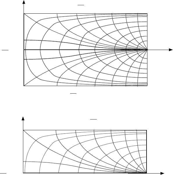
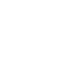
Fig. 4.23

ϕϕ–

ϕ 0=

---–

---

n∂

∂ϕ

n∂

∂ϕ

n∂

∂ϕ

ϕϕ

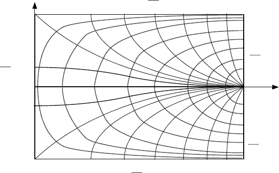
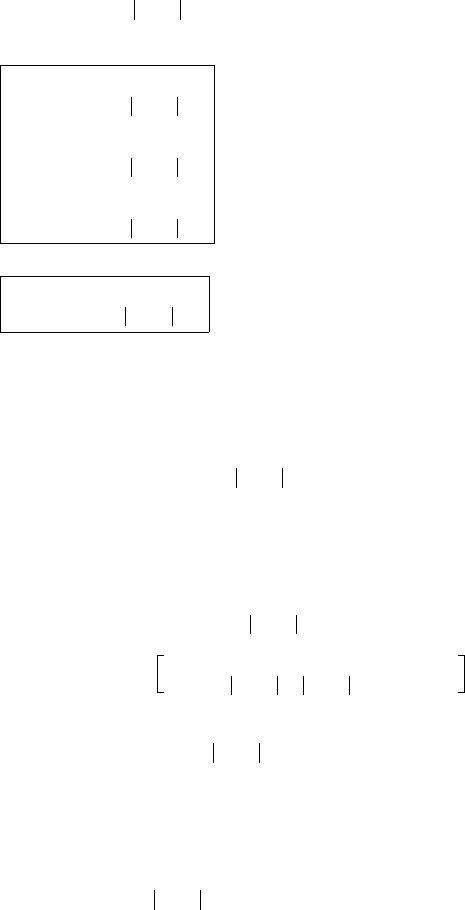
Fig. 4.24

ϕ 0=

---

n∂

∂ϕ

n∂

∂ϕ

ϕϕ

4.5 Some Current Density Fields 255

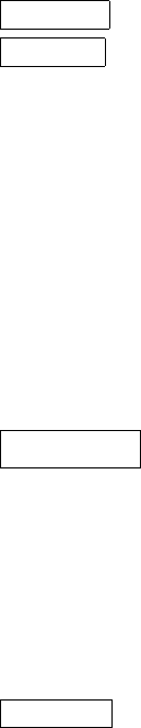
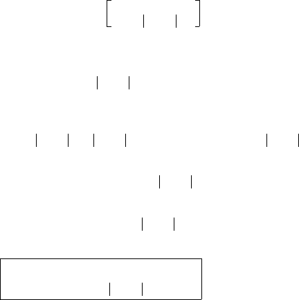
Fig. 4.25

ϕϕ–

---–

---

n∂

∂ϕ

n∂

∂ϕ

n∂

∂ϕ

ϕϕ

ψ 0=

n∂

∂ψ

n∂

∂ψ

ψ 0=

5 Basics of Magnetostatics

5.1 Basic Equations

Maxwell’s equations were introduced in Chapter 1 eq. (1.72). In the limit of just

time-independent problems, the system of Maxwell’s equations nicely splits into

two electrostatic and two magnetostatic equations. The latter consists of Ampere’s

law, and the fact that the magnetic field is always source free (i.e. solenoidal).

(5.1)

. (5.2)

Beyond that, we have to establish a relation between B and H

(5.3)

The relation for vacuum is

(5.4)

The B-field is perceivable because it exhibits a velocity dependent force on

charged particles (Lorentz force). If an electric field exists simultaneously, the force

becomes

(5.5)

Integrating eq. (5.1) over an arbitrary area gives its integral representation

Applying Stokes’s theorem gives

(5.6)

where I is the current through the respective area.

In the following, we calculate the magnetic fields for a variety of

arrangements. Simple cases with a high degree of symmetry allow one to almost

directly write down the magnetic fields from eq. (5.6). However, frequently more

laborious, formal methods need to be applied. This requires the introduction of the

vector potential A. Since the divergence of the curl vanishes for every vector

it is possible to write B in the form

(5.7)

This automatically satisfies eq. (5.2). Any given A uniquely determines B.

Conversely, there are many vector potentials for any given B-field. Obviously,

and

(5.8)

produce the same B-field. The reason is

where for any function the following identity holds

H∇× g =

B∇• 0 =

BBH()=

B µ

F Q EvB×+()=

H∇×()Ad

∫

gAd

∫

H ds•

∫

I =

a∇×()∇• 0=

BA ∇×=

AA' A φ∇+=

A'∇× A∇× φ∇()∇×+ A∇×==

G. Lehner, Electromagnetic Field Theory for Engineers and Physicists,

DOI 10.1007/978-3-540-76306-2_5, © Springer-Verlag Berlin Heidelberg 2010

5.1 Basic Equations 257

Consequently, every B-field can be represented by an infinite number of vector

potentials A. This allows one to impose additional restrictions on A. The proper

choice of satisfies these restrictions, which can be used as a gauge. The

transition from to in eq. (5.8) is termed a gauge transformation of the vector

potential. B remains unchanged and, thus, is said to be gauge invariant. The so-

called Coulomb gauge is very useful for static problems.

(5.9)

For time-dependent problems, the Lorentz gauge is usually used

(5.10)

Its importance will be made clear later.

From eqs. (5.1), (5.4). and (5.7) follows, that for currents in vacuum

Using the vector identity

(5.11)

and eq. (5.9) gives

(5.12)

For Cartesian coordinates we find

(5.13)

where represents the ordinary Laplacian or Laplace operator

The reader shall be cautioned in applying the Laplace operator to vec-

tors, since only for Cartesian coordinates the result is simply an applica-

tion of the double derivative to the individual components. This can

easily be verified by applying the gradient, divergence, and curl in cur-

vilinear coordinates (as we have discussed in Sections 3.1 through 3.3),

and use eq. (5.11) to calculate , i.e.,

It is recommended to eliminate in this way when using curvilinear

coordinates.

φ∇()∇× 0=

AA'

A∇• 0 =

A∇• µε

t∂

∂ϕ

+0 =

H∇×

------

∇×

------

A∇×()∇×

------

A∇×()∇× g====

A∇×()∇× A∇•()∇∇

A– A∇•()∇∆A–==

∇

A µ

g –=

∇

AA∇•()∇ A∇×()∇×–=

∇

r() µ

– r()=

∇

r() µ

r()–=

∇

r() µ

r()–=

∇

258 Basics of Magnetostatics

The equation in cylindrical coordinates is

(5.14)

where again represents the ordinary Laplace operator, whose form is given by

eq. (3.33):

Now we see that it would be wrong to attempt splitting eq. (5.12) in its cylindrical

components and write it in the form

FALSE!

The reason for all this lies in the fact that the basis vectors for curvilinear

coordinates are functions of the location, for instance in cylindrical coordinates

and (not , however), which results in additional terms when differentiating.

In Cartesian coordinates we have

while for cylindrical coordinates we get

where

To calculate the related fields when the currents g(r) are given, requires one

to solve eq. (5.12), which in Cartesian coordinates is represented by the three scalar

equations of (5.13), and for cylindrical coordinates by the three scalar equations

given by (5.14). For formal reasons, we will initially restrict ourselves to Cartesian

coordinates. We know already the solution of the three equations (5.13). These are

three scalar Poisson equations. We have shown in electrostatics that the equation

∇

∂

∂x

--------

∂

∂y

--------

∂

∂z

--------++=

∇

-----

ϕ∂

∂A

-----–– µ

–=

∇

-----

ϕ∂

∂A

------–+ µ

–=

∇

–=

∇

---

r∂

∂

r∂

∂ 1

-----

∂

∂ϕ

---------

∂

∂z

--------++=

∇

–=

∇

–=

∇

–=











∇

A ∇

++()e

∇

++==

∇

A ∇

++()e

∇

A()

∇

A()

∇

A()

++==

∇

A()

∇

≠ , ∇

A()

∇

≠

∇

ϕ r()

ρ r()

-----------–=

5.1 Basic Equations 259

can be solved by the potential (see eq. (2.20))

Similarly, from eq. (5.13) follows:

(5.15)

Of course we may combine these three equations into one vector equation

(5.16)

However, important to remember is that this equation is valid only in Cartesian

coordinates.

What remains to be proven is that the vector potential eq. (5.16) is indeed

source-free, as our gauge (5.9) requires. We find

having used the vector identity

and the fact that g(r’) is independent of the field point r. Furthermore

because for stationary currents

And finally, because of Gauss’ theorem

The reason is that the integral covers the entire space and there will be no currents

crossing a sufficiently distant surface. Note that we use da for the surface element

here and whenever confusion with the vector potential A is possible.

ϕ r()

4πε

------------

ρ r'()

rr'–

---------------

τ'd

∫

r()

4π

------

r'()

rr'–

---------------

τ' d

∫

r()

4π

------

r'()

rr'–

---------------

τ' d

∫

r()

4π

------

r'()

rr'–

---------------

τ' d

∫

Ar()

4π

------

gr'()

rr'–

---------------

τ' d

∫

A∇• r()

4π

------

gr'() ∇

rr'–

---------------

•τ' d

∫

af()∇• a f∇()• f a∇•()+=

A∇• r()

4π

------

gr'()∇

rr'–

---------------

•τ' d

∫

–=

µ–

4π

---------

(∇ ) •

gr'()

rr'–

---------------

rr'–

---------------

(∇ ) •

gr'()– τ'd

∫

A∇• r()

4π

------

(∇ ) •

gr'()

rr'–

---------------

τ' d

∫

g∇• 0=

A∇• r()

4π

------

gr'()

rr'–

---------------

da'•

∫

–0==

260 Basics of Magnetostatics

One needs to beware of a false conclusion, here. We already saw that

when . However, this does not mandate that we select the

Coulomb gauge when dealing with magnetostatic problems, where we have, of

course, . It only means that our approach does not bear any contradiction.

Our assumption was the Coulomb gauge ( ). Any different result would

constitute a contradiction. On the other hand, if we choose current densities that are

not source free ( ), then we end up with a contradiction. Since always

the following must also be true

Therefore, it should not be a surprise that for , we obtain a wrong vector

potential

When choosing a different gauge, then the vector potential calculated for a given

current distribution satisfies this other gauge if and only if .

In principle, this solves the calculation of magnetic fields due to any current

distribution. In an actual case, this may still turn out to be difficult.

Instead of the vector potential, the field may be directly expressed by an

integral. From eqs. (5.16) and (5.7) we obtain

We use

and therefore

(5.17)

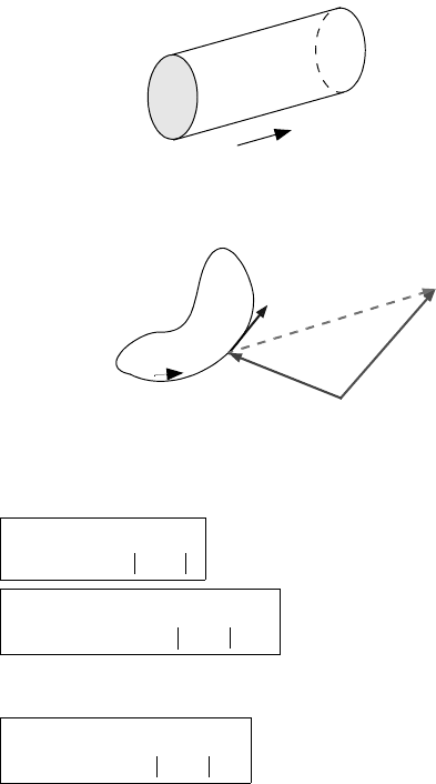
This is the so-called Biot-Savart’s law in its most general form. If there are only

currents in relatively narrow conductors we may approximate (Fig. 5.1)

A∇• 0= g∇• 0=

g∇• 0=

A∇• 0=

g∇• 0≠

A∇×()∇× µ

A∇×()∇×()∇• 0 µ

g∇•==

g∇• 0 .=

g∇• 0≠

A∇• 0≠

g∇• 0=

BA ∇×

4π

------

gr'()

rr'–

---------------

τ'd

∫

∇×==

4π

------

()∇×

gr'()

rr'–

---------------

τ' d

∫

()∇×

gr'()

rr'–

---------------

rr'–

---------------

()∇×

gr'() gr'() ∇×

rr'–

---------------

–=

gr'()

rr'–

------------------

–





×–=

gr'()

rr'–

------------------





×=

B r()

4π

------

gr'() rr'–()×

rr'–

-----------------------------------

τ' d

∫

gr'()dτ' gr'()dA'ds' Ids'==

5.1 Basic Equations 261

This changes eqs. (5.16) and (5.17) to now read

(5.18)

. (5.19)

These integrals extend over the entire, closed current loop or all the closed current

loops (Fig. 5.2). Frequently, it is said that the line element creates the field

(5.20)

Often, this is also called the Biot-Savart law. Unfortunately, this form is

mistakable, we might almost say even wrong. Indeed, the field expressed by

eq. (5.20) is a possible field, as it is source free. The related current density field is

obtained from

Taking the divergence on both sides reveals that it is always source free:

However, the current I in the line element is not source free. This constitutes an

apparent contradiction. Nevertheless, the correct current density field can be

calculated immediately. To simplify and make this easier to understand, just

assume that the line element is located at the origin and is oriented along the

positive z-axis. When using spherical coordinates, dB and dH have only a ϕ-

component

Fig. 5.1

gr'()

dA'

ds'

Ar()

4π

--------

s'd

rr'–

---------------

∫

Br()

4π

--------–

rr'–()ds'×

rr'–

------------------------------

∫

ds'

4π

--------–

rr'–()ds'×

rr'–

------------------------------

gH∇×=

g∇• H∇×()∇• 0==

Fig. 5.2

ds'

rr'–

ds'

262 Basics of Magnetostatics

This makes

We know the electrostatic analogue of this field very well. It represents the dipole

field given by eq. (2.63). Thus, it describes the current I within a line element with

the point-like isotropic current sources +I at its upper end and -I at its lower end,

that is, a “dipole current density” which occupies the entire space. It is rotationally

symmetric. Therefore, by using Ampere’s law, one can show that this flux exactly

causes the given magnetic field. It is furthermore apparent that all positive and

negative point sources cancel each other when integrating over a closed contour,

thereby leaving only the current I in the closed conductor. This explanation

plausibly clarifies the integral result (5.19), which we had obtained in a purely

formal manner.

To go beyond the current magnetostatic treatment of this problem and to

regard it as time dependent problem is also possible. Currents with sources are now

permissible, which however, requires time dependent volume charges, because of

the charge conservation (continuity equation). Besides the magnetic field, one

needs to consider also time dependent electric fields and thereby displacement

current densities, i.e., the current densities above are replaced by displacement

current densities. We will not elaborate on this subject here.

To use the Biot-Savart law in its integral form (5.19) is advisable in

magnetostatics. Nevertheless, the differential form can be used as well, if

interpreted in the correct way, as just outlined.

Oftentimes, the vector potential is very useful to calculate the magnetic flux.

Because of

and using Stokes’ theorem we obtain:

(5.21)

The vector potential was introduced as an auxiliary quantity to calculate B. At

this point it is frequently said that only B has real meaning, while A has no

significance beyond its role as an auxiliary quantity. This is not correct because in

quantum mechanics, the field A is necessary and is a real field. The experiment by

Bohm and Aharonov, interpreted in a quantum mechanical way shows for example,

that the A field is important in certain regions (e.g., outside of infinitely long coils,

Ids' θsin

4πr

--------------------=

dg dH∇×

Ids'

4πr

------------

2 θcos=

Ids'

4πr

------------

θsin=

0 .=











φ Bad•

∫

∇ A×()ad•

∫

φ As d•

∫

5.1 Basic Equations 263

see Section 5.2.3), where even when , the A field remains . The

Bohm-Aharonov experiment shall not be discussed here. Details can be found in

Appendix A.3.

Besides the vector potential, there is also a scalar magnetic potential, whose

usefulness is restricted to describe magnetic fields in regions that are current free.

If in a region , then

Therefore, H can be obtained from a scalar potential by taking the gradient (note

that here is not related to the previously discussed flux function).

(5.22)

is a unique function in a simply connected region and shares most

properties with the electric potential . When multiply connected regions enclose

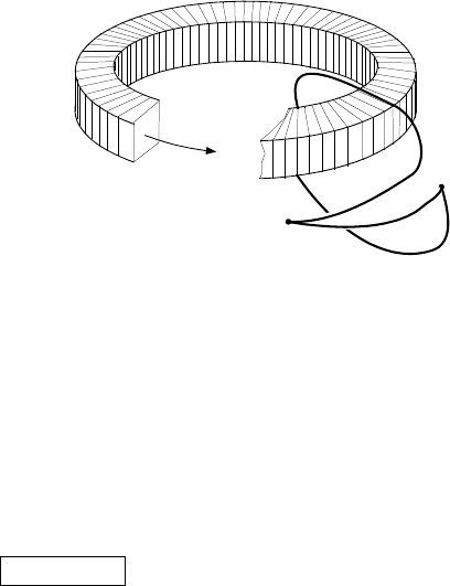
currents, becomes ambiguous (Fig. 5.3). Consider a current carrying toroidal

region. We pick the two points A and B in the current-free space and the two

different paths C

and C

, both starting at A and ending at B. Together C

and C

enclose the current carrying region. Ampere’s law (5.6) states

that is

More generally, we could be interested in a path that loops n times around the

current I (Fig. 5.4). Then we get

(5.23)

B 0= A 0≠

g 0=

H∇× 0=

H ψ ∇–=

Fig. 5.3

H ds•

∫

()

H ds•

∫

()

+ I =

H ds•

∫

()

H ds•

∫

()

I– =

H ds•

∫

()

H ds•

∫

()

nI– =