Lehner G. Electromagnetic Field Theory for Engineers and Physicists

Подождите немного. Документ загружается.

544 Numerical Methods

The discretization described above is not the only one possible. It is also

possible to obtain more accurate relations when one includes more points during

the discretization. For example, consider the Laplace operator. We start with a one-

dimensional function , where for example,

or as well

Adding gives

Analogously we find

Mixing the last two relations by using the weights a and b gives

(8.164)

Choosing and gives

(8.165)

Proceeding in an analogous way for the second derivatives gives

(8.166)

and with and

(8.167)

For the one-dimensional case, eq. (8.167) is already a five-point formula, i.e., in

order to express ϕ’’, it uses the values of ϕ at five points. Analogously, for the two-

and three-dimensional case, this results in 9 or 13 point formulas. The best value

for a and b in each case is determined by the remainder term of the Taylor

expansion, which should be of the highest possible order (i.e. as small as possible).

More details are provided for example, by Marsal [19]. Another interesting

ϕ x()

i 1+

–

-----------------------

≈

i 1–

–

-----------------------

≈

i 1+

i 1–

–

-------------------------------

≈

i 2+

i 2–

–

-------------------------------

≈

2a ϕ

i 1+

i 1–

–()b ϕ

i 2+

i 2–

–()+

4ha b+()

----------------------------------------------------------------------------------------

≈

a 4= b 1–=

8 ϕ

i 1+

i 1–

–()ϕ

i 2+

i 2–

–()–

12h

---------------------------------------------------------------------------------

≈

i 1+

2ϕ

– ϕ

i 1–

----------------------------------------------

≈

i 2+

2ϕ

– ϕ

i 2–

----------------------------------------------

≈

4a ϕ

i 1+

i 1–

+()b ϕ

i 2+

i 2–

+()24ab+()ϕ

–+

ab+()

----------------------------------------------------------------------------------------------------------------------------

≈

a 4= b 1–=

16 ϕ

i 1+

i 1–

+()ϕ

i 2+

i 2–

+()–30ϕ

–

12h

------------------------------------------------------------------------------------------------------

≈

8.6 Method of Finite Differences 545

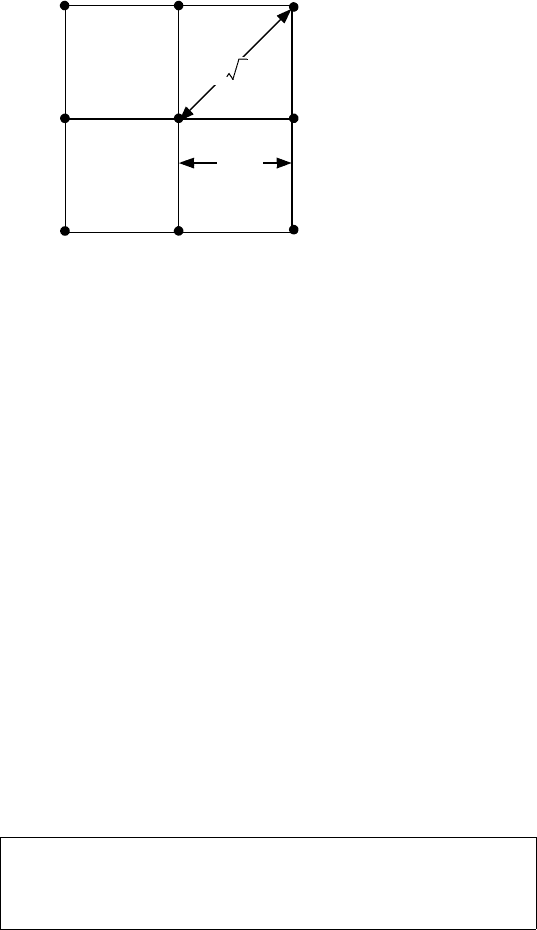
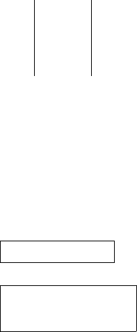
representation of the two-dimensional Laplace operator is the following.

According to eq. (8.156) for the nine gridpoints presented in Fig. 8.8 , we have

and also

Therefore

and with ,

(8.168)

In particular for

(8.169)

Further details and similar relations can also be found in Marsal [19].

Fig. 8.8

i 1+ j,

ij 1–,

i 1– j,

ij 1+,

ij,

h 2

i 1+ j 1–,

i 1– j 1–,

i 1– j 1+,

i 1+ j 1+,

∇

ij,

i 1+ j,

i 1– j,

ij 1+,

ij 1–,

4ϕ

ij,

–+++

------------------------------------------------------------------------------------------------------

≈

∇

ij,

i 1+ j 1+,

i 1+ j 1–,

i 1– j 1+,

i 1– j 1–,

4ϕ

ij,

–+++

------------------------------------------------------------------------------------------------------------------------------------

≈

2a ϕ

i 1+ j,

i 1– j,

ij 1+,

ij 1–,

+++()

∇

ij,

b+ ϕ

i 1+ j 1+,

i 1+ j 1–,

i 1– j 1+,

i 1– j 1–,

+++()42ab+()ϕ

ij,

–

ab+()

-----------------------------------------------------------------------------------------------------------------------------------------------------------------------------

≈

a 2= b 1=

4 ϕ

i 1+ j,

i 1– j,

ij 1+,

ij 1–,

+++()

∇

ij,

i 1+ j 1+,

i 1+ j 1–,

i 1– j 1+,

i 1– j 1–,

+++()20ϕ

ij,

–+

--------------------------------------------------------------------------------------------------------------------------------------------------------

≈

∇

ϕ 0=

4 ϕ

i 1+ j,

i 1– j,

ij 1+,

ij 1–,

+++()

ij,

i 1+ j 1+,

i 1+ j 1–,

i 1– j 1+,

i 1– j 1–,

+++()+

-----------------------------------------------------------------------------------------------------------------------------------

≈

546 Numerical Methods

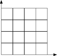
8.6.2 An Example

As an example, we shall apply the method to the Dirichlet boundary value problem

depicted in Fig. 8.9. There are nine gridpoints inside the square area. The Laplace

equation shall be solved for the boundary conditions of at the top

boundary and at the remaining boundaries (all are dimensionless

quantities)

Its solution is

(8.170)

where d represents the sides of the square. Evaluating this result at the gridpoints

yields the following potentials:

(8.171)

The following approximations can be compared with these results.

The five-point formula (8.159) yields the following six equations:

(8.172)

Solving it directly yields

(8.173)

ϕ 100=

ϕ 0=

400

---------

---

nπy

---------





sinh

nπx

---------





sin

nπ()sinh

--------------------------------------------------

n 135…,,,=

∑

43.20833 ,= ϕ

54.052922 ,= ϕ

18.202833 ,=

25 ,= ϕ

6.797166 ,= ϕ

9.541422=

---

–

---

– 25=

---

– ϕ

---

– 25=

---

– ϕ

---

–

---

– 0=

---

–

---

– ϕ

---

– 0=

---

– ϕ

---

– 0=

---

–

---

– ϕ

+ 0=











300

--------- 42.85== ,ϕ

1475

------------ 52.67 ,==

------ 18.75 ,== ϕ

25 ,=

------7.14 ,== ϕ

275

---------9.82 .==











8.6 Method of Finite Differences 547

Of course, these values deviate from the exact ones, but the maximum error is just

under 5%.

One can also apply the nine-point formula (8.169). This requires to use the

potentials at the corners of the square. At the discontinuities (i.e. at ,

and at , ), one has to use the average, i.e. . This gives the

following equations:

(8.174)

and its solutions

(8.175)

This coincides astonishingly well with the exact solutions eq. (8.170) and (8.171),

respectively. The maximal error is at about 0.1%, and thereby about 50 times

Fig. 8.9

ϕ 0=

ϕ 100=

x 0= yd=

xd= yd= ϕ 50=

---

–

---

–

------

–

------=

---

– ϕ

------

–

---

– 30=

---

–

------

– ϕ

---

–

---

–

------

– 0=

------

–

---

–

---

– ϕ

------

–

---

– 0=

---

–

------

– ϕ

---

– 0=

------

–

---

–

---

– ϕ

+ 0=











25.159

---------------- 4 3 . 2 0 6 5== ,ϕ

25.1095

506

------------------- 5 4 . 1 0 0 7 ,==

200

--------- 18.1818 ,== ϕ

25 ,=

625

--------- 6.7934 ,== ϕ

25.193

506

---------------- 9 . 5 3 5 5 .==











548 Numerical Methods

smaller than when using the five-point formula. The exact value for the potential

is obtained in both cases.

The so-called Gaussian elimination is oftentimes used for the direct solution

of the systems of equations, whereby the coefficient matrix is transformed into a

triangular matrix by applying elementary row operations. This results in an easily

solvable system of equations. Another method is the so-called LR decomposition

(“left-right decomposition”). In this case, the matrix is transformed into a product

of two triangular matrices, which also allows to conveniently solve the system of

equations.

Oftentimes the system is solved iteratively. For this purpose, one uses

estimations for the potentials at the gridpoints. Then, by means of the respective

formulas, one calculates new values etc., i.e. from the potentials of the n-th

iteration steps ( ) one calculates the values of the (n+1)-th step ( ) as

follows:

(8.176)

This is the so-called Jacobi method. Convergence of the iteration is accelerated in

case of the Gauss-Seidel method. Here, in step (n+1), not only the old values n are

used, but already the new values of the step (n+1) are used as much as they are

available. Further acceleration of the convergence can be achieved through the

relaxation method, which shall only be mentioned here, but not further discussed.

Of course, the iteration converges better, if the initial estimates are more

accurate. At least for the current example, it is easy to find very useful estimates by

using the five-point formula or – what amounts to the same – using the mean value

theorem. Consider initially only an inner gridpoint in the center, then based on the

boundary values one estimates a value of . Now one narrows the grid

according to Fig. 8.9. From and the boundary values, the corners in particular,

one obtains an estimate for and , namely and

. This allows one to estimate the remaining potentials,

, , . Now, based on these values one iterates by use

of eq. (8.176). It remains left for the reader to convince himself, that this converges

towards the approximations given in (8.173), but not towards the exact value. The

Gauss-Seidel method accelerates the convergence. In contrast to the Jacobi

method, the symmetry of the values for the potential of the present problem is

initially lost, even though this will, of course, finally converge towards the

symmetric approximation solution.

These proceedings may be modified in many ways. The grid spacing for the

various coordinate directions may be chosen with different values. The lattice does

not need to be uniform, i.e. the grid may be variable inside a region. This leads to

the method of local grid refinement, if inside a particular region an extremely fine

discretization is needed in order to achieve a required accuracy.

Of course, the method of finite differences is applicable to all sorts of

differential equations. Space or time dependent problems (for example diffusion

equations or wave equations), generally require one to also discretize the time.

25=

ij,

n()

ij,

n 1+()

ij,

n 1+()

---

i 1+ j,

n()

i 1– j,

n()

ij 1+,

n()

ij 1–,

n()

+++()=

0()

25=

0()

175 4 44≈⁄=

0()

25 4 6≈⁄=

0()

53= ϕ

0()

19= ϕ

0()

8.7 Finite Elements Method 549

Depending on the strategy, there are two different types of difference equations. In

the first case, the so-called explicit methods, all quantities of a given “time plane”

are calculated from the immediately preceding time plane. In the second case, the

implicit methods, the equations of one time plane contain the unknowns of the

subsequent time plane. This distinction is of importance because the per se simpler

explicit methods exhibit the disadvantage that they may be unstable, i.e. that errors

may grow and the numerical results become useless. This only seemingly

insignificant difference shall be illustrated by means of the example of the

diffusion equation. We may discretize the equation

(8.177)

in the form

(8.178)

but also in the form

(8.179)

In case of the explicit formulation (8.178), all can be directly calculated from

the values , generally all from etc. In contrast, the implicit

formulation (8.179) requires more computing effort. The so-called semi-implicit

methods constitute a compromise between the two methodologies whereby the two

relations (8.178) and (8.179) are mixed by the weight factors α and 1 - α (“Euler

factor”).

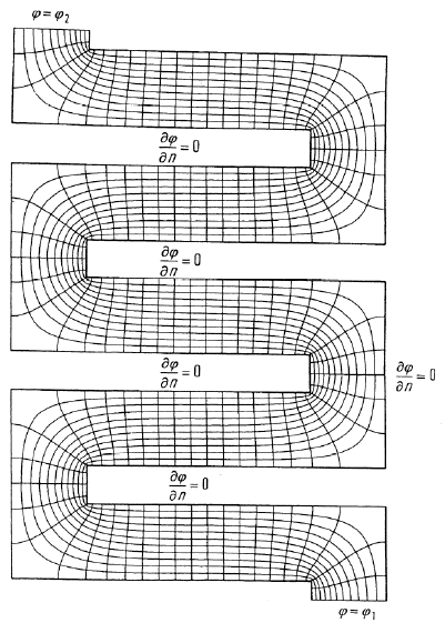
As an example, Fig. 8.10 shows the current density field inside a meandering

thin-film resistor, which was calculated by means of the finite difference method.

This is a two-dimensional, mixed boundary value problem ( and

at the two contacts on top and bottom, at the other boundaries). For

this example, the domain decomposition method was additionally used. This

allows one to reduce such a problem to finding the solutions in subregions, where

the boundary conditions at the additional boundaries need to be initially estimated.

The problem is then solved iteratively. More details on this method can be found in

Bader [20]. In the present case, the area was partitioned entirely in rectangles.

8.7 Finite Elements Method

The method of Finite Elements has quickly gained significance. Although the

effort in any particular application may be substantial, the method is in principle

based on a simple and elegant idea. It is very flexible and thereby applicable to

many types of problems. Oftentimes, it is superior to other methods, although this

may not be the case for every type of problem. Corresponding to its significance,

∂

∂x

--------- A

∂u

∂t

------

i 1– k,

ik,

– u

1 i+ k,

--------------------------------------------------------- A

ik 1+,

ik,

–

∆t

-------------------------------

i 1– k 1+,

ik 1+,

– u

1 i+ k 1+,

-------------------------------------------------------------------------------- A

ik 1+,

ik,

–

∆t

-------------------------------

ik,

i 0,

ik 1+,

ik,

ϕϕ

= ϕϕ

∂ϕ ∂n⁄ 0=

550 Numerical Methods

the available literature covering finite elements is rather extensive. As examples,

the books [17, 19, 21 through 27] shall be mentioned.

For this method, the region of definition of the unknown function or functions

is partitioned into more or less arbitrarily shaped domains – just the finite elements,

partial lines, partial surfaces, partial volumes, depending on the dimension of the

region that needs discretization. Every finite element is associated with an

approximate solution which is non vanishing only inside of that element. The

approximate solution consists of a set of linearly independent basis functions (the

so-called form functions) and a corresponding number of initially undetermined

parameters. These parameters represent the value of the function itself, which it

assumes at certain points of the finite element, the so-called nodal points. These

nodal points, thereby, play a similar role as the gridpoints did in case of the finite

difference method. The not so insignificant difference is based on the fact that the

approximate solution assumed in the finite element method, approximates the

unknown function at all points, not only at the nodal points. On the other hand, the

method of finite difference may be regarded as a special case of the method of

finite elements. Furthermore, even in case of the finite difference method, it is

possible by proper interpolation, to assign values to all points The entire region has

Fig. 8.10

8.7 Finite Elements Method 551

to be filled with finite elements in such a way that every node at the boundary of a

finite element coincides with the node of its neighbor elements, whereby the value

of the functions have to match there as well. Together with the boundary

conditions, one obtains a system of equations that allows to determine the value of

the function at the nodal points. Thereby, one starts either with the method of the

weighted residuals, usually in the form of the Galerkin method or – given the

variational integral exists – one starts from the Rayleigh-Ritz method, which is

equivalent to the Galerkin method.

Before providing more in depths details, we will illustrate what we have

learned so far by a two-dimensional example. A particularly simple one-

dimensional example that highlighted some of the important steps was already

provided in Sect. 8.4.5, equations (8.128) and following. In the two-dimensional

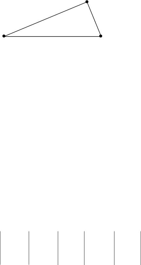
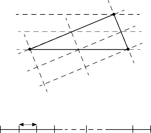
case, triangles can be used as finite elements, which need to fill the entire area.

Fig. 8.11 shows one of these triangles with the corners and the

corresponding values . The corners constitute the nodal points. Inside

the triangle, we attempt to approximate the unknown function by a function of the

form

(8.180)

Then, for every corner or nodal point, it has to be

a, b, c can be calculated from these three equations:

,, ,

(8.181)

where D is the coefficient determinant.

Fig. 8.11

,()

ϕ abxcy++=

abx

,++= i 123,,=

----

= b

----

1 ϕ

= c

----

1 x

552 Numerical Methods

(8.182)

If one lets

(8.183)

then for these so-called form functions we have

(8.184)

and the Ansatz (8.180) takes the form

(8.185)

Together with eq. (8.184) we obtain, as necessary:

(8.186)

This means that eq. (8.185) represents the Ansatz within the observed finite

element, in form of a linear combination of the form function and the coefficients

represent the values of the function at the nodal points. These functions are non-

vanishing only inside this particular finite element. The Ansatz for the problem

overall, is finally obtained by superposition of all trial functions of all elements.

The form function can also be interpreted as being so-called triangular coordinates.

Every point in a triangle can be determined by the triangle coordinates .

As indicated in Fig. 8.12 , these are defined in such a way that the side opposite of

is associated with and the line parallel to it that cuts through is the

line . On the parallel lines inbetween, takes on distance proportional

values. Of course, two of these three triangular coordinates are sufficient to

uniquely characterize a point. The relation between the triangular coordinates and

Cartesian coordinates is given by the coordinates of the corner points. We have

(8.187)

From this, one obtains for example, for the point with , ,

just , , etc. Since the relation has to also be linear, it is

1 x

xy,()

----

–()y

–()xx

–()y++[]=

xy,()

----

–()y

–()xx

–()y++[]=

xy,()

----

–()y

–()xx

–()y++[]=

,()δ

ϕϕ

xy,()

i 1=

∑

,()

i 1=

∑

i 1=

∑

===

0= P

1= ξ

x ξ

++=

y ξ

++=

1 ξ

++=











1= ξ

0= xx

= yy

8.7 Finite Elements Method 553

thereby proven. If one now calculates the triangular coordinates

corresponding to a point x, y, then one precisely obtains the form functions

(8.188)

The form functions thereby also represent a local coordinate system on the

corresponding triangle. This knowledge is useful when calculating many of the

integrals that are necessary when applying, for example, the Galerkin or the

Rayleigh-Ritz method.

The described triangles, together with the linear form functions (8.183) and

the related Ansatz (8.185) provide only a simple example. Practical applications

use two- and three-dimensional finite elements of different types, with a varying

number of nodal points and oftentimes much more complicated form functions of

higher order. The details may become very voluminous and may be expressed in a

complicated form, which of course, does not change the basically simple and

elegant principle.

To simplify, the procedure shall be illustrated by means of the one-

dimensional example which we have already mentioned in Sect. 8.4.5. Consider

the region and partition it as shown in Fig. 8.13 in n finite elements of

length

(8.189)

with the nodal points , where

Fig. 8.12

---=

xy,()f

xy,()=

≤≤

Fig. 8.13

n 1–

x–

----------------=

i 0 …n,=()