Lehner G. Electromagnetic Field Theory for Engineers and Physicists

Подождите немного. Документ загружается.

534 Numerical Methods

and we will also use a different set of basis functions, namely

(8.128)

and

(8.129)

This Ansatz represents a piecewise linear approximation of the function values

between the locations . The values of the

functions occur as coefficients of the particular basis functions. The basis functions

are each different from zero only in one of the subregions. This is a simple example

of the method of finite elements, which we will discuss later in detail. Here, we

chose special and very simple (namely linear) form functions.

It is now possible to use the Galerkin method or the Rayleigh-Ritz method to

calculate u

and u

are given by the boundary conditions), which has to

lead to the same result as before. In case of the Galerkin method, the residue

contains the second derivative of u, . According to eq. (8.129), the first

derivatives u’ are discontinuous at the sampling points. This means that the second

derivatives are δ-functions. The necessary integrals can be calculated by means of

these δ-functions. These integrals can be avoided when integrating by parts

(8.130)

This situation is referred to as the “weak” formulation of the problem. We will use

the variational method, which only needs u’(x) from start, that is, it represents the

weak formulation from the beginning. The calculation is tedious but without any

problems and yields

(8.131)

and

u 0() u

= u 1() u

13x–()u

3xu

+ for 0 x 13⁄≤≤

23x–()u

3x 1–()u

+for13⁄ x 23⁄≤≤

33x–()u

3x 2–()u

+for23⁄ x 1≤≤











3 u

–()for 0 x 13⁄≤≤

3 u

–()for 1 3⁄ x 23⁄≤≤

3 u

–()for 2 3⁄ x 1 .≤≤











,,, x 01 3⁄ 23⁄ 1,,,=

∇

uu''=

ux()u'' x()xd

∫

u' x()[]

∫

– ux()u' x()[]

Iu' x()[]

ux()+{}xd

∫

–2u

–+++()=

---





---

25u

------

++ +





8.4 Method of Weighted Residuals 535

(8.132)

i.e.

(8.133)

The exact solution of the problem is

(8.134)

This means that at the two sampling points, we obtain the exact value for u

and u

We get the intermediate values by linear interpolation. For the special case

we find

(8.135)

Written in a slightly different form, the two eqs. (8.132) read

(8.136)

This exhibits great similarity with the result obtained by means of the finite

differences (as we shall see later). For , one obtains from eq. (8.162) of

the upcoming Section 8.6.1 the following result:

(8.137)

The difference between them manifests itself in the right sides of the equations,

which stems from the inhomogeneity . Eqs (8.137) give

∂I

∂u

-------- 6 u

–12u

–7

---





++0==

∂I

∂u

-------- 6 u

–12u

–25

---





++0==











---

------

---





–+=

---

------

---





.–+=

–

------–





------

++=

0==

486

---------– ,= u

486

---------–=

– u

---





– u

------

---















h 13⁄=

– u

+ h

---





---





– u

+ h

---





---















536 Numerical Methods

(8.138)

and for

(8.139)

Now, we have approximated solutions of eq. (8.112) with the boundary condition

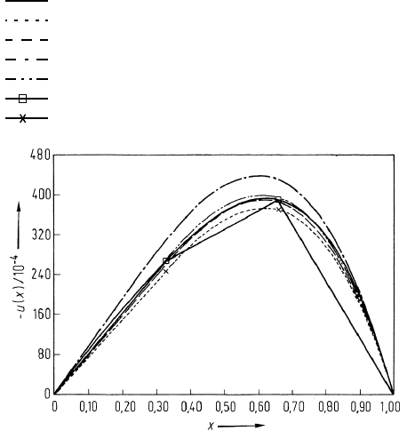
(8.113) by many different ways. Fig. 8.3 compares the exact solution (8.114) with

the various approximations, namely:

• Eq. (8.117) Collocation

• Eq. (8.122) Overdetermined Collocation

• Eq. (8.124) Method of Fractional Regions, Momentum Method,

Method of Least Error Squares

• Eq. (8.127) Galerkin Method, Rayleigh-Ritz Method

• Eq. (8.135) Rayleigh-Ritz Method with different trial functions

• Eq. (8.139) Method of finite differences.

---





–+=

---





–+=











0==

------– ,= u

------–=

Fig. 8.3 Comparison of exact solution with various approximations

Exact Solution

Collocation Method

Overdetermined Collocation

Fractional Regions, Momentum Method, Least Error Squares

Galerkin, Variation

Finite Elements

Finite Differences

8.5 Random-Walk Processes 537

Fig. 8.3 clearly illustrates that the various solutions are of different quality. On the

other hand, it also becomes clear that by means of only a few simple trial functions,

one can obtain very useful approximations. Nevertheless, one should not jump to

conclusions with respect to the quality of the various methods based on

generalizations of the results depicted in Fig. 8.3.

The method of the weighted residuals may be used in various variants. With

the exception of the Monte-Carlo method, it can be regarded as the starting point of

all the numerical methods which we will discuss in the following, namely the

method of finite differences, the method of finite elements, boundary element

method, and the method of image charges. Only the Monte-Carlo method is based

on an entirely different approach. Nevertheless, for the field theoretical problems

which we consider here, this method is ultimately equivalent to the method of finite

differences.

8.5 Random-Walk Processes

In anticipation of the Monte-Carlo method, we consider simple random-walk

processes. These are special, stochastic processes, which represent a very useful

and intuitive model for many theoretical, and in practice interesting problems

within the Theory of Probability and in Physics.

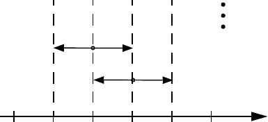
We start from a one-dimensional discrete random-walk process. For this purpose,

consider an infinitely long straight line with equidistant grid points, which we

identify by whole numbers from through (Fig. 8.4). At time , a

particle (or a person) shall be located at point 0. Within defined time intervals, the

particle moves in steps towards the right or left, each direction with the probability

or q, respectively. Of course,

(8.140)

We want to know what is the probability to find the particle at any particular

location after n steps. The probability to be at location after n steps is, we

claim

∞– ∞+

Fig. 8.4

-3 -2 -1 1 20

step 1

step 2

t 0=

q+1=

2mn–

538 Numerical Methods

(8.141)

In order to arrive at point requires to move m of the total n steps to the right

and steps to the left. The order of the steps is immaterial. The m and the

steps, respectively, may be selected from the n steps in different ways.

Remarkable is that because of eq. (8.140):

(8.142)

Therefore, the function is called the generating function of the

probabilities w. Eq. (8.142) can be explained plausibly by the fact that when

expanding , the occurrence of the product is the same as picking

m or n-m elements of the total number of n elements, when disregarding the order.

This explains the relation to the probabilities. At the same time, eq. (8.142) reveals

that the sum of the probabilities equals 1, as it must be.

To know the generating function is very helpful. Consider, for example, the

average of the passed locations after n steps and the average of its square:

(8.143)

From eq. (8.142) follows that

and

Therefore

(8.144)

. (8.145)

Adding the two equations gives

(8.146)

2mnn,–

nm–





2mn–

nm–





pq+()

nm–





m 0=

∑

1 ===

pq+()

nm–

x〈〉 2mn–()





nm–

m 0=

∑

〈〉 2mn–()





nm–

m 0=

∑











pq+()

np q+()

n 1–

m 1–

nm–





m 0=

∑

n== =

pq+()

nn 1–()pq+()

n 2–

mm 1–()p

m 2–

nm–





m 0=

∑

nn 1–() .=

nm–





m 0=

∑

np=

mm 1–()p

nm–





m 0=

∑

nn 1–()p

nm–





m 0=

∑

nn 1–()p

np+=

8.5 Random-Walk Processes 539

Using eqs. (8.144) and (8.146) one finds

(8.147)

. (8.148)

For the symmetric random-walk process one has and

(8.149)

. (8.150)

Symmetry explains the vanishing of . Eq. (8.150) is very interesting. If the

steps occur at equidistant points in time, then . The square root of the

squared average of the surpassed distance is thus proportional to , and not to t.

This is a typical property of diffusion processes, which can be regarded as

generalized random-walk processes. We already discovered this fact, while

covering the diffusion equation in Sect. 6.2.3, eq. (6.39) in particular. Of course, for

the limit (or ), because in this case all the steps proceed in only one

direction – either left or right – we obtain:

(8.151)

This represents a directed motion and not a random-walk.

From a purely formal perspective, the random-walk problem may be treated

as the solution to a difference equation for probabilities. Let be the probability

that after k steps, a particle is found at location i. Then

(8.152)

The methods to solve such difference equations are entirely analogous to the

solution of differential equations. Both require initial and boundary conditions in

order to make the solutions unique. The probabilities given above (8.141) satisfy

the difference equations. They represent their only solution for the infinite one-

dimensional space when the probabilities vanish at infinity and the initial condition

(8.153)

Conversely, one might want to analyze finite regions which limit the possible

motion of the particle and note for example, that a particle arriving at or

is absorbed or reflected, respectively (or absorbed or reflected with a certain

probability). Based on difference equations, boundary conditions, and initial

conditions one can calculate the various probabilities on a one-, two-, or three-

dimensional lattice. This constitutes a wide field with many interesting results,

which we shall not discuss here. However, when solving field theoretical problems

by means of the Monte-Carlo method, then one-, two-, or three-dimensional

discrete and symmetric random-walk processes with absorbing walls will be

applied.

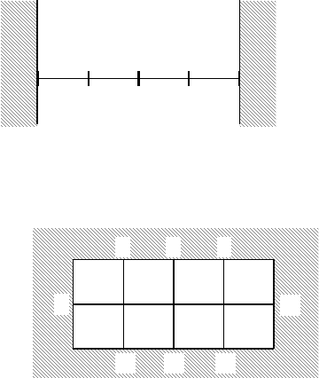
Here, we consider a few simple probabilities that will be required later.

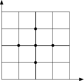
Fig. 8.5 shows a finite, one-dimensional lattice with absorbing walls at 0 and 4, and

with three internal points. Let a particle carry out a random-walk process starting at

x〈〉 n 2p 1–() =

〈〉 n

2p 1–()

4np 1 p–() +==

q 12⁄==

x〈〉 0 =

〈〉 n ,= x

〈〉 n=

x〈〉

nt∼

x〈〉 n± x

〈〉, n

ik,

i 1– k 1–,

i 1+ k 1–,

i 0,

ia=

ib=

540 Numerical Methods

one of the inner points. We ask, what is the probability W

for a particle starting at

point i to be absorbed at point k, if k is a boundary point or, how often it passes the

point k, if it is an inner point. The reader may convince himself that the

probabilities are as follows:

(8.154)

When we include the “passing” of the initial point, this would make ,

, .

In case of the two (three) dimensional symmetric random-walk, the particles

move with the equal probability of 1/4 (1/6), respectively, towards one of the four

(six) neighboring points. Fig. 8.6 shows a simple two-dimensional lattice with

absorbing walls. What is the probability W

for a particle starting at point i, to be

absorbed at point k? Note that this question, unlike above, does not ask for the

frequency of passing inner points. Initially, to simplify, we note that there are only

three significant boundary points. Because of symmetry, the probabilities of being

absorbed at 4, 4’, or 4’’ are the same. The same is true for 5 and 5’’, as well as for 6,

6’, and 6’’. Furthermore, and this is left for the reader to verify, we have

Fig. 8.5

12034

---

,= W

---

,= W

1= , W

---= , W

---=

---= , W

1= , W

---=

---= , W

1 ,= W

---

,= W

---=











32⁄=

2= W

32⁄=

Fig. 8.6

1203

4’

4’’ 5’’ 6’’

6’

5 6

8.6 Method of Finite Differences 541

(8.155)

Of course it must be

and so on.

8.6 Method of Finite Differences

8.6.1 Fundamental Relations

The method of finite differences is one of the oldest numerical methods. The

procedure shall be illustrated by using the Poisson equation as an example. To

simplify, we start from a rectangular region and use Cartesian coordinates x, y (i.e.,

we consider a two-dimensional problem). As shown in Fig. 8.7 , the area is

“discretized”, i.e. only the potentials that occur at the corners of small squares

at the gridpoints , will be considered. The side of these squares have the

length h. Expanding into a Taylor series gives

------

, == W

------

,== W

------==

------

,== W

------











+1=

++ 1=

Fig. 8.7

i 1+ j,

ij 1–,

i 1– j,

ij 1+,

ij,

542 Numerical Methods

Adding these four equations while disregarding the terms of higher order gives

(8.156)

and with the Poisson equation

(8.157)

. (8.158)

For , this results in the so-called five-point formula

(8.159)

It interlinks the potentials at the five points shown in Fig. 8.7. It expresses the

potential at each gridpoint (not at the boundary points) in terms of the mean value

of the potentials at its four neighbor points. Because of the corresponding mean

value theorem (8.38), this is not surprising. If one regards the gridpoint with the

potential ϕ

i,j

as the center of a circle with radius h, then the current approximation

of the potentials on the circumference are represented by the potentials at the four

mentioned points, whose averaging gives the potential at the center. The five-point

formula is nothing less than the corresponding two-dimensional mean value

theorem in a discretized form.

This can easily be generalized to three-dimensional problems by analogously

defined gridpoints x

, y

, z

. Each gridpoint now has six neighboring points.

Expanding this in a Taylor series gives now six, instead of the previous four

addends. Their summation gives

(8.160)

For , i.e., for the Laplace equation, this leads to the seven point formula

i 1+ j,

ij,

∂ϕ

ij,

∂x

------------

---

∂

ij,

∂x

--------------

0 h

()++ +=

i 1– j,

ij,

∂ϕ

ij,

∂x

------------

h–

---

∂

ij,

∂x

--------------

0 h

()++=

ij 1+,

ij,

∂ϕ

ij,

∂y

------------

---

∂

ij,

∂y

--------------

0 h

()++ +=

ij 1–,

ij,

∂ϕ

ij,

∂y

------------

h–

---

∂

ij,

∂y

--------------

0 h

()++=

4ϕ

ij,

∇

ij,

+ ϕ

i 1+ j,

i 1– j,

ij 1+,

ij 1–,

+++≅

∇

ij,

–=

ij,

---

i 1+ j,

i 1– j,

ij 1+,

ij 1–,

+++()

ij,

--------------

+≅

g 0=

ij,

---

i 1+ j,

i 1– j,

ij 1+,

ij 1–,

+++() ≅

ijk,,

---

i 1+ jk,,

i 1– jk,,

ij 1 k,+,

ij 1 k,–,

ijk 1+,,

ijk 1–,,

+++++()≅

ijk,,

------------------

g 0=

8.6 Method of Finite Differences 543

(8.161)

This represents the three-dimensional mean value theorem, eq (8.36), in discrete

form.

For the one-dimensional case we have of course

(8.162)

and for

(8.163)

For comparison purposes, we have already used eq (8.162) in a previous section –

eq. (8.137), , .

Writing the corresponding equation, i.e., one of eqs. (8.158) through (8.163),

depending on the kind of problem, for every internal gridpoint of a one- or two-

dimensional lattice, then one obtains a linear system of algebraic equations. For the

Laplace equation, it is homogeneous. When prescribing the potential at the

boundary, this results in a solvable inhomogeneous system of equations with a

unique solution. The number of equations is equal to the number of grid points

inside and thereby equal to the number of unknowns (that is, the potentials at the

inner gridpoints). One can prove that the coefficient matrix exhibits the necessary

properties (that is, its determinant does not vanish). This reveals that the

uniqueness theorem, proven in the potential theory for the solution of the Dirichlet

boundary value problem (Sect. 3.4.3), because of the discretization, is related to the

theorems of linear algebra.

The solution to Neumann or mixed boundary value problems is similar, but

more tedious, and will not be discussed here.

The given relations need to be adopted in case of arbitrarily shaped

boundaries, which requires to adjust the varying distances of the gridpoints from

the boundary (“boundary region formulas”), which adds to complicating matters.

This too, will be skipped here.

In any case, for all such problems, one obtains uniquely solvable systems of

linear equations. To solve a pure Neumann boundary value problem requires one to

fix a constant, for example, by prescribing the potential at a gridpoint. The results

become increasingly accurate (within certain limits) as the granularity decreases,

i.e., the smaller the lattice constant h is chosen. Of course, this increases the

computing effort as the number of unknowns increases. An advantage is thereby

that the obtained coefficient matrix is only lightly populated, that is, it consists of

mostly vanishing elements. The voluminous systems of equations can either be

solved directly (for example, by Gauss elimination, by left-right decomposition,

etc.) or by means of iteration methods (for example, Jacobi method, Gauss-Seidel

method, or the relaxation method, etc.)

ijk,,

---

i 1+ jk,,

i 1– jk,,

ij 1 k,+,

ij 1 k,–,

ijk 1+,,

ijk 1–,,

+++++()≅

---

i 1+

i 1–

+()

----------

+≅

g 0=

---

i 1+

i 1–

+() ≅

h 13⁄= gx

–=