Marder M.P. Condensed Matter Physics

Подождите немного. Документ загружается.

Magnetic Dipole Moments

733

0 100 200 300 400 500 600 700

Temperature T (K)

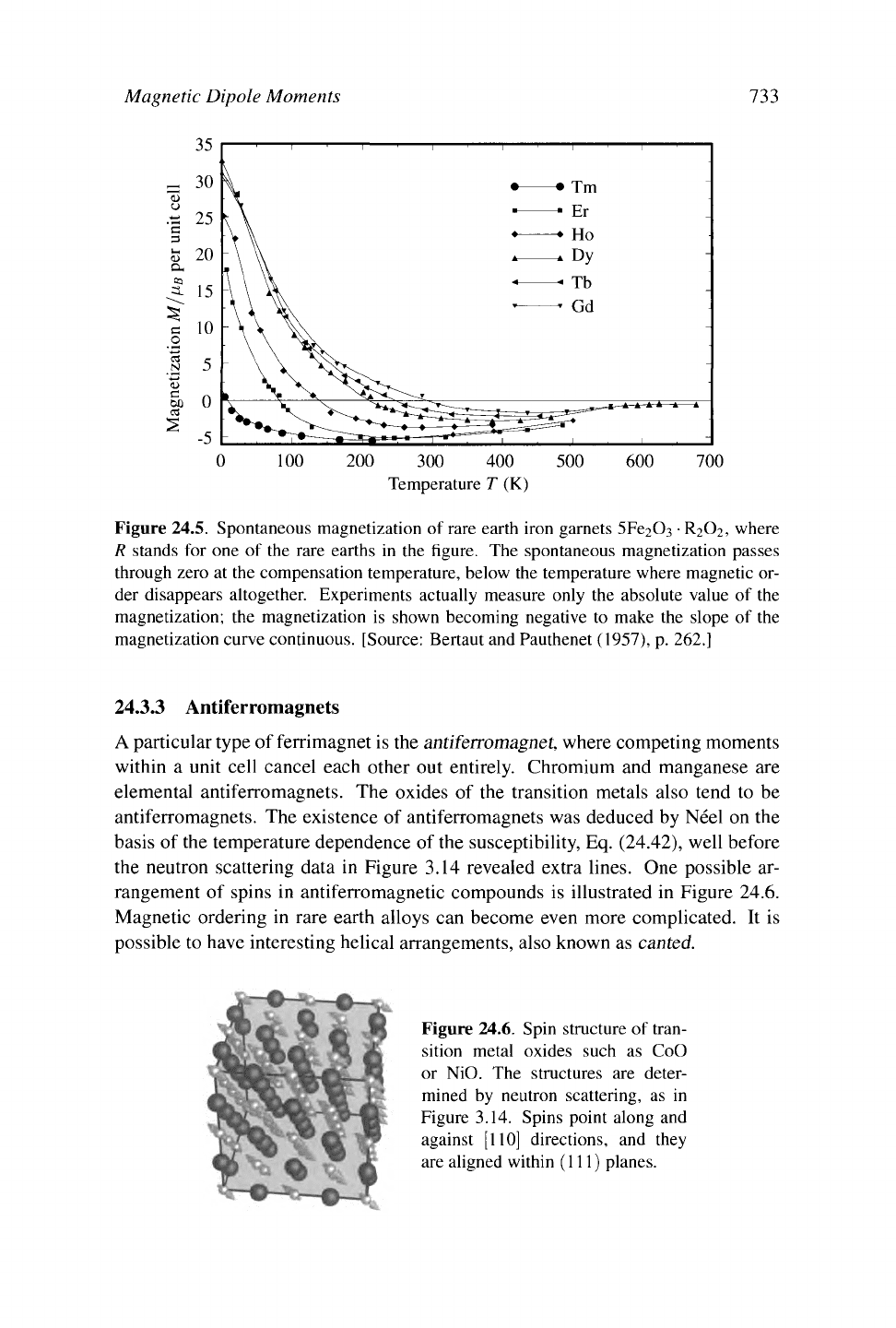
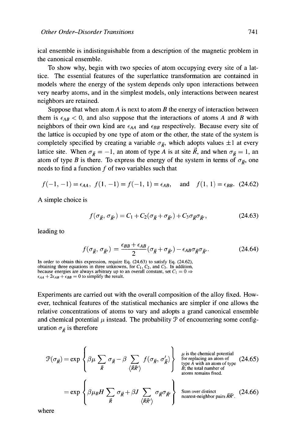
Figure 24.5. Spontaneous magnetization of rare earth iron garnets 5Fe2Û3 R2O2, where

R stands for one of the rare earths in the figure. The spontaneous magnetization passes

through zero at the compensation temperature, below the temperature where magnetic or-

der disappears altogether. Experiments actually measure only the absolute value of the

magnetization; the magnetization is shown becoming negative to make the slope of the

magnetization curve continuous. [Source: Bertaut and Pauthenet (1957), p. 262.]

24.3.3 Antiferromagnets

A particular type of ferrimagnet is the antiferromagnet, where competing moments

within a unit cell cancel each other out entirely. Chromium and manganese are

elemental antiferromagnets. The oxides of the transition metals also tend to be

antiferromagnets. The existence of antiferromagnets was deduced by Néel on the

basis of the temperature dependence of the susceptibility, Eq. (24.42), well before

the neutron scattering data in Figure 3.14 revealed extra lines. One possible ar-

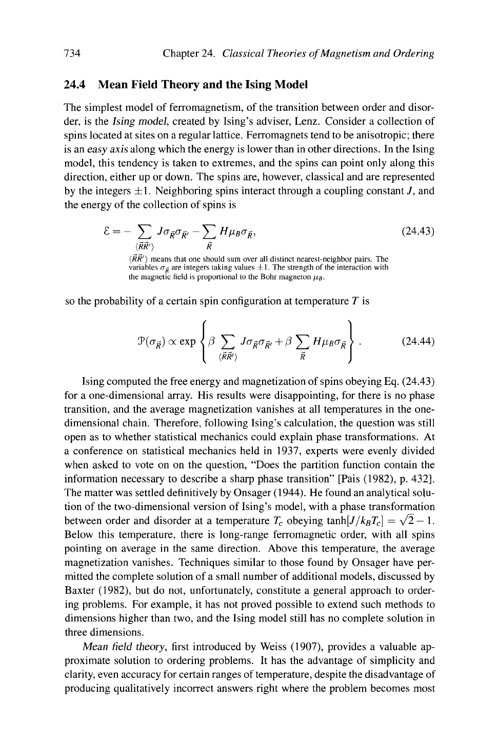
rangement of spins in antiferromagnetic compounds is illustrated in Figure 24.6.

Magnetic ordering in rare earth alloys can become even more complicated. It is

possible to have interesting helical arrangements, also known as

canted.

Figure 24.6. Spin structure of tran-

sition metal oxides such as CoO

or NiO. The structures are deter-

mined by neutron scattering, as in

Figure 3.14. Spins point along and

against [110] directions, and they

are aligned within (111) planes.

734

Chapter 24. Classical Theories of Magnetism and Ordering

24.4 Mean Field Theory and the Ising Model

The simplest model of ferromagnetism, of the transition between order and disor-

der, is the Ising model, created by Ising's adviser, Lenz. Consider a collection of

spins located at sites on a regular

lattice.

Ferromagnets tend to be anisotropic; there

is an easy axis along which the energy is lower than in other directions. In the Ising

model, this tendency is taken to extremes, and the spins can point only along this

direction, either up or down. The spins are, however, classical and are represented

by the integers ±

Neighboring spins interact through a coupling constant J, and

the energy of the collection of spins is

£ = - Y.

°R

~ E

«> <

)

(RR'} R

(RR'} means that one should sum over all distinct nearest-neighbor pairs. The

variables a^ are integers taking values ±

The strength of the interaction with

the magnetic field is proportional to the Bohr magneton ßß-

so the probability of a certain spin configuration at temperature T is

7(a

) oc exp ^ ß ^ Ja

,+ß ^ Hfi

(RR') R

(24.44)

Ising computed the free energy and magnetization of spins obeying Eq. (24.43)

for a one-dimensional array. His results were disappointing, for there is no phase

transition, and the average magnetization vanishes at all temperatures in the one-

dimensional chain. Therefore, following Ising's calculation, the question was still

open as to whether statistical mechanics could explain phase transformations. At

a conference on statistical mechanics held in 1937, experts were evenly divided

when asked to vote on on the question, "Does the partition function contain the

information necessary to describe a sharp phase transition" [Pais (1982), p. 432].

The matter was settled definitively by Onsager (1944). He found an analytical solu-

tion of the two-dimensional version of Ising's model, with a phase transformation

between order and disorder at a temperature T

obeying tanh[J / kßT

] = \/2— 1.

Below this temperature, there is long-range ferromagnetic order, with all spins

pointing on average in the same direction. Above this temperature, the average

magnetization vanishes. Techniques similar to those found by Onsager have per-

mitted the complete solution of a small number of additional models, discussed by

Baxter (1982), but do not, unfortunately, constitute a general approach to order-

ing problems. For example, it has not proved possible to extend such methods to

dimensions higher than two, and the Ising model still has no complete solution in

three dimensions.

Mean field theory, first introduced by Weiss (1907), provides a valuable ap-

proximate solution to ordering problems. It has the advantage of simplicity and

clarity, even accuracy for certain ranges of temperature, despite the disadvantage of

producing qualitatively incorrect answers right where the problem becomes most

Mean Field Theory

and

the Ising Model 735

interesting,

in the

vicinity

of the

phase transition.

The

idea

is to

replace

sys-

tem

interacting spins

by a

single spin sitting

in the

mean,

average, magnetic

field produced

by all its

neighbors. This average magnetic field

calculated

self-

consistently

asking what magnetic field

the

single spin must produce when

sits

in a

uniform external field

and by

demanding that

the two

fields agree.

The

qualitative error

this calculation

is the

neglect

correlations.

For

example,

near

phase transition, magnetic spins aggregate into blobs

spins pointing

in the

same direction, while different blobs point in different

ways.

The average magnetic

field may

zero while simultaneously

the

chance

of a

spin

and its

near neighbors

pointing

in the

same direction

very high. Mean field theory cannot correctly

characterize this situation, because

if the

average field

zero, mean field theory

predicts

correlation between

spin

and its

neighbors.

Formally, mean field theory proceeds

observing that

the

difficulty

com-

puting

partition function resulting from Eq. (24.43) lies

in the

products

spins

cr^cr^,, and that the partition function could immediately be summed if only

single

power

the spin appeared. Write

°R

= a + \?R ~ v)

is the

average spin.

(24.45)

and treat (er^

—

a) as

formally

small quantity. Then, keeping

up to

first order

this supposedly small quantity, one obtains

(

(°R>

)]

-o{a

+ a

,)-a

-2

(24.46)

Let

z, the

coordination number,

be the

number

nearest neighbors with which

each spin interacts, and

N be the

total number

spins. Then

- E

R ~

NzJ(J

-Y^{H

+ H)ß

(24.47)

Use Eq. (24.46)

for

cr^a^,.

H is the

mean field seen

each spin, produced

its neighbors.The factor

of 1/2 in the

first term comes from

the

restriction

distinct nearest-neighbor pairs.

with

zJu

The partition function

Z for

the spin system

can

therefore

written

Z«

\-ß{NzJ(T

/2-Y,{H + H)ß

)

a\...ON

-ßNzJä

exp[ß{H

H)ii

]

exp[-ß(H

H)/i

}

(24.48)

(24.49)

(24.50)

^J=-k

In Z =

NzJâ

/2-Nk

T ln[2 cosh ßß

{H + H)}. (24.51)

To close

the

mean field theory,

one has to

determine

the

mean field

H, or

equiva-

lent^

the

mean spin

ä. The

mean spin

^=7

E 7?E

exp[-/3£

}}

^ N'

O\...UN

(24.52)

736 Chapter 24. Classical Theories of Magnetism and Ordering

= - V ———exp[-/3£ {a A] See

Eq.

(24.43). (24.53)

Z ^ ßNu

FL H x RIS

= Because

=-k

TlaZ.

(24 54)

N fi

= tanh/3/iß (// + //) Employing the approximation of

Eq.

(24.51). (24.55)

=>■

ä = tanh ß[zJä + ß

H}. (24.56)

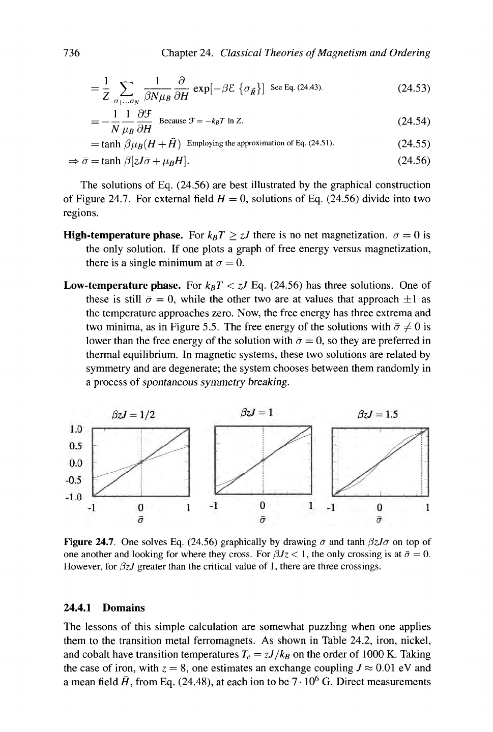
The solutions of Eq. (24.56) are best illustrated by the graphical construction

of Figure 24.7. For external field H = 0, solutions of Eq. (24.56) divide into two

regions.

High-temperature phase. For kßT > zJ there is no net magnetization, a

—

0 is

the only solution. If one plots a graph of free energy versus magnetization,

there is a single minimum at a = 0.

Low-temperature phase. For kßT < zJ Eq. (24.56) has three solutions. One of

these is still ä = 0, while the other two are at values that approach ±1 as

the temperature approaches zero. Now, the free energy has three extrema and

two minima, as in Figure 5.5. The free energy of the solutions with ä / 0 is

lower than the free energy of the solution with a = 0, so they are preferred in

thermal equilibrium. In magnetic systems, these two solutions are related by

symmetry and are degenerate; the system chooses between them randomly in

a process of spontaneous symmetry breaking.

Figure 24.7. One solves Eq. (24.56) graphically by drawing a and tanh ßzJä on top of

one another and looking for where they cross. For ßJz < 1, the only crossing is at ä = 0.

However, for ßzJ greater than the critical value of

there are three crossings.

24.4.1 Domains

The lessons of this simple calculation are somewhat puzzling when one applies

them to the transition metal ferromagnets. As shown in Table 24.2, iron, nickel,

and cobalt have transition temperatures T

= zJ/kß on the order of 1000 K. Taking

the case of iron, with z = 8, one estimates an exchange coupling J « 0.01 eV and

a mean field H, from Eq. (24.48), at each ion to be 7

•

G. Direct measurements

Mean Field Theory and the hing Model

131

of the field were discussed in Section 13.5, and they are in fact about

3 •

G. But

even after adopting the smaller number, such fields seem exceptionally large on two

counts. First, the magnetization of iron can be made to alter through application of

external fields that are comparatively small, only on the order of

G. It is hard to

understand how iron could be affected by such small fields when vastly larger ones

are operating internally. Second, referring back to Section 22.2, it is somewhat

hard to see how spontaneous magnetization is supposed to arise at all. According

to the calculations of that section, in a spherical region filled with a cubic array of

dipoles, the net field acting upon each dipole due to all the other dipoles is zero. The

arguments referred to electrical dipoles, but nothing changes if magnetic dipoles

appear instead. Ferromagnetic order is supposed to arise because of interactions

between nearby spins, but if the interactions have the form of dipole fields they

cancel each other out completely.

The explanation of these two puzzles is that two rather different types of forces

operate between magnetic moments. At very short distances, on the order of atomic

spacings, magnetic order is induced by powerful exchange forces that arise quan-

tum mechanically from the competition of Coulomb repulsion with Fermi statis-

tics.

This local ordering can be ferromagnetic, antiferromagnetic, ferrimagnetic, or

of a more complicated canted type. Simultaneously, at distances large compared

with atomic spacings, magnetic moments interact as dipoles, with an energy that

falls off as

between any two dipoles, but that can diverge if one sums over all

the interactions between a large population.

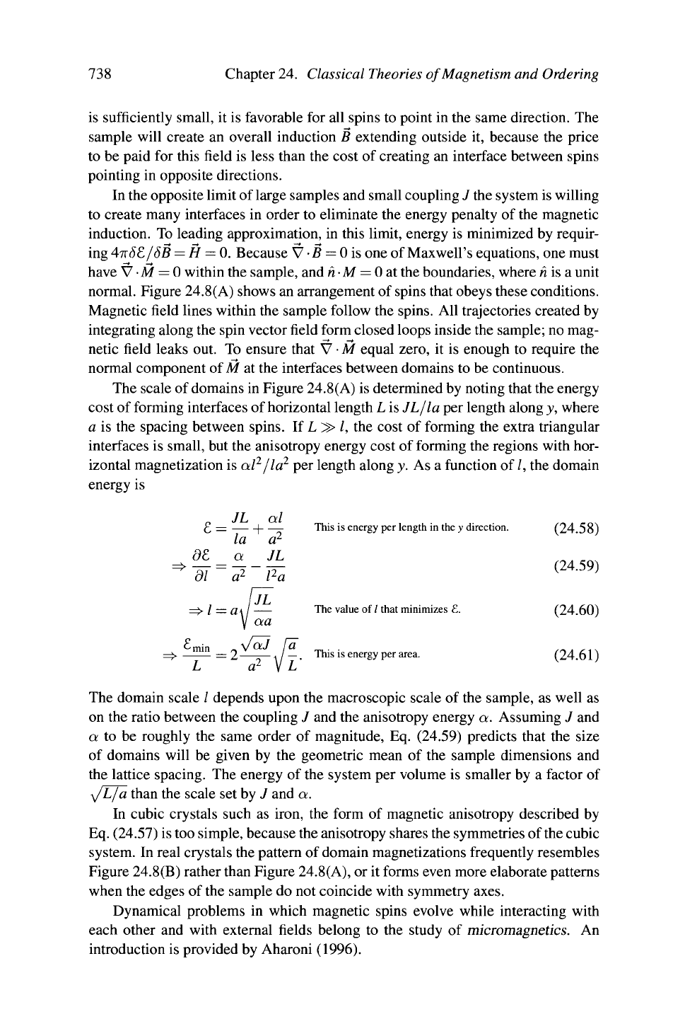
In order to accommodate these two competing interactions, ferromagnets or-

ganize into domains, as depicted in Figure 24.8. The first theory for the size and

shape of the domains is due to Landau and Lifshitz (1935). The simplest context

in which to study them is a model similar to the Ising model. In the Ising model,

spins can point only along the easy axis, a condition too restrictive to permit the

study of

domains.

However, domain structures, as shown in Figure 24.8(B), can be

captured by spins pointing along four directions, x,

—x,

y, and

—y.

Suppose that

the easy axis is still present, and also suppose that spins pointing along ±x have an

energy a per spin greater than spins pointing along ±y. Finally, because domains

emerge from the competition between long- and short-range forces, the magnetic

induction B created by all the spins needs to be included as well. The energy of the

spins is therefore

£ = - J2

°R-VR>

+ Y1 [a(o"

-x)

-fi

B-â

+— j drB-fl. (24.57)

(RR

) R

= ±x or ±)>, and B is the spatially varying magnetic induction created by the

magnetization

M = /xg<r.

Because H =

B-4TTM,

ATZ

SE./SB = H as it should according to Eq. (24.17),

if the sum over R is interpreted as an integral for the purposes of computing the

functional derivative.

Depending upon the size of the coupling constant J, the system will minimize

its energy in different ways. When the coupling constant J is large and the system

738 Chapter 24. Classical Theories of Magnetism and Ordering

is sufficiently small, it is favorable for all spins to point in the same direction. The

sample will create an overall induction B extending outside it, because the price

to be paid for this field is less than the cost of creating an interface between spins

pointing in opposite directions.

In the opposite limit of large samples and small coupling J the system is willing

to create many interfaces in order to eliminate the energy penalty of the magnetic

induction. To leading approximation, in this limit, energy is minimized by requir-

ing 4irô£/ÔB = H = 0. Because V

•

B = 0 is one of Maxwell's equations, one must

have V

•

M = 0 within the sample, and h

•

M = 0 at the boundaries, where « is a unit

normal. Figure 24.8(A) shows an arrangement of spins that obeys these conditions.

Magnetic field lines within the sample follow the spins. All trajectories created by

integrating along the spin vector field form closed loops inside the sample; no mag-

netic field leaks out. To ensure that V

•

M equal zero, it is enough to require the

normal component of M at the interfaces between domains to be continuous.

The scale of domains in Figure 24.8(A) is determined by noting that the energy

cost of forming interfaces of horizontal length L is JL/la per length along y, where

a is the spacing between spins. If L 3> /, the cost of forming the extra triangular

interfaces is small, but the anisotropy energy cost of forming the regions with hor-

izontal magnetization is al

/la

per length along y. As a function of /, the domain

energy is

This is energy per length in the y direction. (24.58)

(24.59)

The value of / that minimizes £. (24.60)

This is energy per area. (24.61 )

The domain scale / depends upon the macroscopic scale of the sample, as well as

on the ratio between the coupling J and the anisotropy energy a. Assuming J and

a to be roughly the same order of magnitude, Eq. (24.59) predicts that the size

of domains will be given by the geometric mean of the sample dimensions and

the lattice spacing. The energy of the system per volume is smaller by a factor of

\jLfa than the scale set by J and a.

In cubic crystals such as iron, the form of magnetic anisotropy described by

Eq. (24.57) is too simple, because the anisotropy shares the symmetries of the cubic

system. In real crystals the pattern of domain magnetizations frequently resembles

Figure 24.8(B) rather than Figure 24.8(A), or it forms even more elaborate patterns

when the edges of the sample do not coincide with symmetry axes.

Dynamical problems in which magnetic spins evolve while interacting with

each other and with external fields belong to the study of micromagnetics. An

introduction is provided by Aharoni (1996).

Mean Field Theory and the hing Model 739

(A)

(B)

Figure 24.8. (A) Domain formation in a rectangular bar magnet. Notice that the flux

lines form closed loops, so no flux escapes from the bar, because the normal component of

the magnetic induction is continuous across the domain boundaries. (B) In an anisotropic

crystal, domain structures become more complicated. While domains orient themselves so

as to reduce the amount of flux that escapes the crystal, they also follow crystalline axes,

and some small domains produce magnetic fields outside the sample.

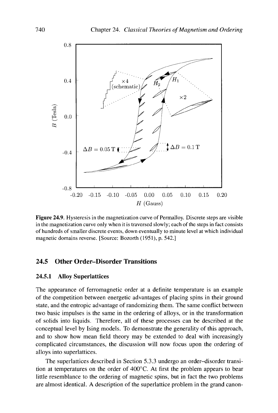
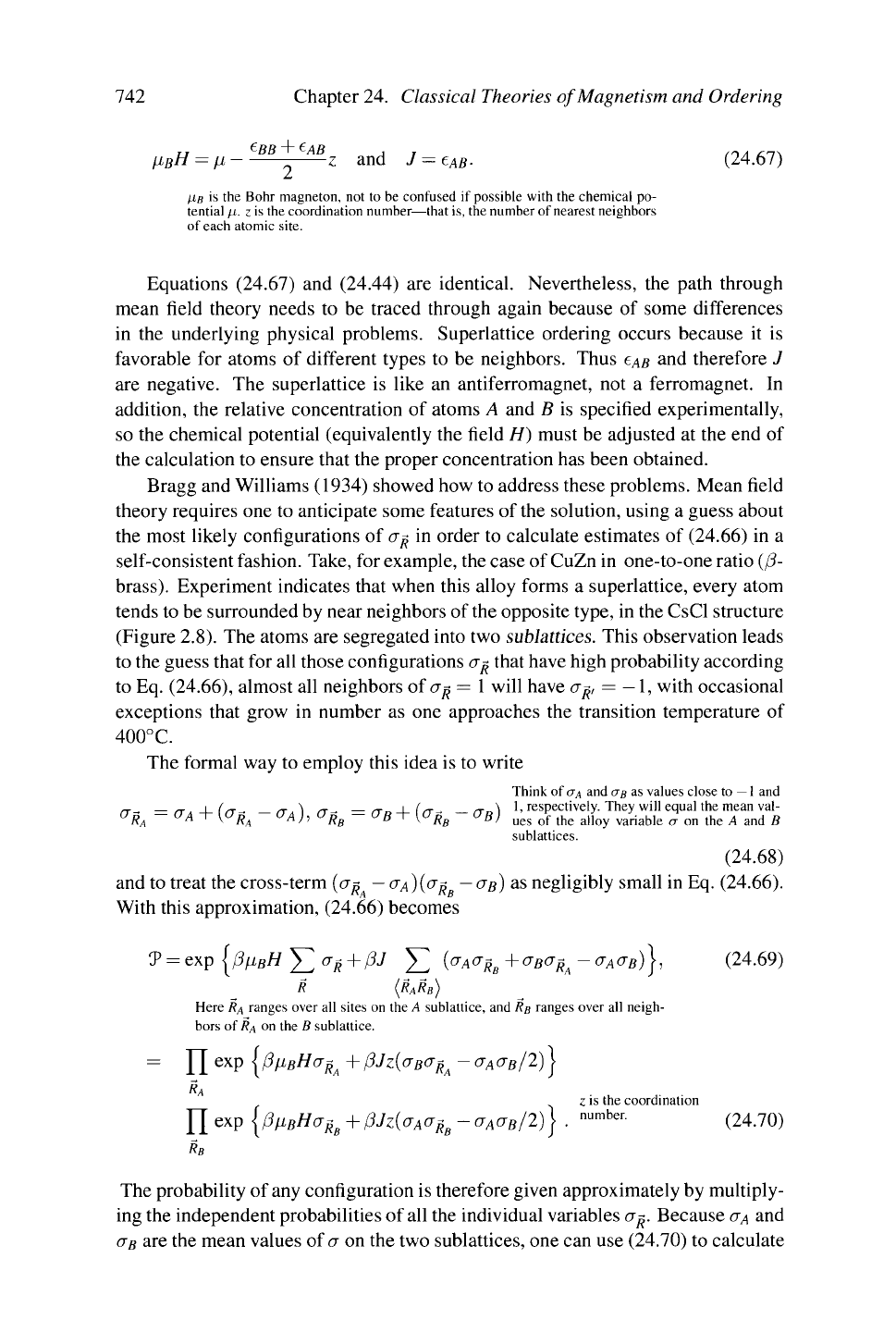
24.4.2 Hysteresis

As shown in Figure 24.9, changing an external magnetic field by 0.05 G can alter

the induction of a ferromagnetic sample by 0.1 T. Compared to internal fields of

300 kG, the applied field seems negligible. The reason for the large measurable

effect is that external fields cause changes in the sizes and orientations of domains,

rather than ripping apart the local magnetic order. The dynamics of the domains

are complicated, and their states depend in detail upon the particular history of

fields that has been applied to them. Figure 24.9 illustrates the hysteretic relation

between B and H as an applied field is increased or decreased in various ways.

An interesting phenomenon illustrated in Figure 24.9 is return-point memory.

If H is increasing and then the direction is reversed at H\, the magnetic field B

decreases along a shallower path than it had during the initial rise. Reversing H at

H2 so that it rises again, B follows yet a third path until H reaches H\ again, where

B changes slope to follow the original curve. One explanation for this phenomenon

appears in Problem 8.

740

Chapter 24. Classical Theories of Magnetism and Ordering

0.8

-0.20 -0.15 -0.10 -0.05 0.00 0.05 0.10 0.15 0.20

H (Gauss)

Figure

24.9.

Hysteresis in the magnetization curve of

Permalloy.

Discrete steps are visible

in the magnetization curve only when it

traversed slowly; each of the steps

fact consists

hundreds

of smaller discrete

events,

down eventually to minute level at which individual

magnetic domains reverse. [Source: Bozorth (1951), p. 542.]

24.5 Other Order-Disorder Transitions

24.5.1 Alloy Superlattices

The appearance of ferromagnetic order at a definite temperature is an example

of the competition between energetic advantages of placing spins in their ground

state,

and the entropie advantage of randomizing them. The same conflict between

two basic impulses is the same in the ordering of alloys, or in the transformation

of solids into liquids. Therefore, all of these processes can be described at the

conceptual level by Ising models. To demonstrate the generality of this approach,

and to show how mean field theory may be extended to deal with increasingly

complicated circumstances, the discussion will now focus upon the ordering of

alloys into superlattices.

The superlattices described in Section 5.3.3 undergo an order-disorder transi-

tion at temperatures on the order of 400°C. At first the problem appears to bear

little resemblance to the ordering of magnetic spins, but in fact the two problems

are almost identical. A description of the superlattice problem in the grand canon-

Other Order-Disorder Transitions 741

ical ensemble

indistinguishable from

description of the magnetic problem in

the canonical ensemble.

To show why, begin with two species

atom occupying every site

of a

lat-

tice.

The essential features

the superlattice transformation are contained

models where the energy

the system depends only upon interactions between

very nearby atoms, and in the simplest models, only interactions between nearest

neighbors are retained.

Suppose that when atom A is next to atom B the energy of interaction between

them

EAB

0, and also suppose that the interactions

atoms

and

with

neighbors

their own kind are

EAA

and

EBB

respectively. Because every site of

the lattice is occupied by one type of atom or the other, the state of the system

completely specified by creating

variable a^, which adopts values ±1

every

lattice site. When

a^ =

—1,

an atom of type A

is at

site R, and when

—

atom of type

is there. To express the energy of the system in terms

ag, one

needs to find a function

of two variables such that

f(-l,-l) = e

, /(l,-l)=/(-l,

l) =

and /(l,

. (24.62)

A simple choice is

)

= C

l +

(<7jj

+ 0>

)

O$0ft,

(24.63)

leading to

r, N £BB + £AB, . s

J{VR,

VR>)

= ~

K^R

+ ^R'l-^AB^Rfrft-

(24.64)

In order

obtain this expression, require Eq. (24.63)

satisfy Eq. (24.62),

obtaining three equations

three unknowns, for C\, C2, and C3.

addition,

because energies are always arbitrary up to an overall constant, set C\

= 0

=S>

£A4

2EAB

ess

0 to simplify the result.

Experiments are carried out with the overall composition of the alloy fixed. How-

ever, technical features

the statistical mechanics are simpler

one allows the

relative concentrations

atoms

vary and adopts

grand canonical ensemble

and chemical potential

instead. The probability

of encountering some config-

uration a^ is therefore

. ß is the chemical potential

9(<Tg)

= exp i ßa V ag - ß V f(a

, a'

) } for replacing an

atom

of (24.65)

RJ r \rr /_^ R ^ J \ RI R) i

with an atom of

type

where

type A with an atom of type

(ÜR

) I

B; the total number of

atoms remains fixed.

exp

ßßBH

R (M')

> Sum over distinct

_ (24.66)

nearest-neighbor pairs RR'.

742

Chapter 24. Classical Theories of Magnetism and Ordering

H = [i z and J = e

. (24.67)

is the Bohr magneton, not to be confused if possible with the chemical po-

tential

ß.

is the coordination number—that is, the number of

nearest

neighbors

each atomic

site.

Equations (24.67) and (24.44) are identical. Nevertheless, the path through

mean field theory needs to be traced through again because of some differences

in the underlying physical problems. Superlattice ordering occurs because it is

favorable for atoms of different types to be neighbors. Thus

CAB

and therefore J

are negative. The superlattice is like an antiferromagnet, not a ferromagnet. In

addition, the relative concentration of atoms A and B is specified experimentally,

so the chemical potential (equivalently the field H) must be adjusted at the end of

the calculation to ensure that the proper concentration has been obtained.

Bragg and Williams (1934) showed how to address these problems. Mean field

theory requires one to anticipate some features of the solution, using a guess about

the most likely configurations of a^ in order to calculate estimates of (24.66) in a

self-consistent fashion. Take, for example, the case of CuZn in one-to-one ratio (ß-

brass).

Experiment indicates that when this alloy forms a superlattice, every atom

tends to be surrounded by near neighbors of the opposite type, in the CsCl structure

(Figure 2.8). The atoms are segregated into two sublattices. This observation leads

to the guess that for all those configurations a^ that have high probability according

to Eq. (24.66), almost all neighbors of a$ =

will have a^, =

—

with occasional

exceptions that grow in number as one approaches the transition temperature of

400°C.

The formal way to employ this idea is to write

Think

of a

and

<xg

as values close to

—

and

\ I

rr \ rr n

-i-( rr

rr \

'■

respectively.

They will equal the mean val-

—°^^~\°R

°^>^

—°B^-\

°ß^ ues of the alloy variable a on the/I and ß

sublattices.

(24.68)

and to treat the cross-term (a^

—

)(a^

—

&B)

as negligibly small in Eq. (24.66).

With this approximation, (24.66) becomes

7 = exp {ßp

H ^a^ + ßJ ^ {°AG$

°AOB)},

(24.69)

R {R

RB)

Here

ranges over all sites on the A sublattice, and

ranges over all neigh-

bors

of R

on the B sublattice.

Yl exp lyßiißHa^ +ßJz(a

-a

/2)j

is the coordination

J] exp {ßn

+ ßJz(a

äe

- a

/2)} .

number

- (24.70)

The probability of any configuration is therefore given approximately by multiply-

ing the independent probabilities of all the individual variables a^. Because a

and

are the mean values of a on the two sublattices, one can use (24.70) to calculate