Masujima M. Applied Mathematical Methods in Theoretical Physics
Подождите немного. Документ загружается.


9.7 The Second Variation 337
The function U(x) r epresents another infinitesimal change in the solution to the
Euler equation which would also pass through x = x
1
.Since
U(x
1
) = U(ξ) = 0, (9.7.37)
there exists another solution u(x)suchthat
u(x) = 0forx ∈ (x
1
, ξ ). (9.7.38)
We choose x
3
such that
x
2
< x
3
<ξ (9.7.39)
and another solution u(x)tobe
u(x) = u
1
(x)u
2
(x
3
) − u
1
(x
3
)u
2
(x), u(x
3
) = 0. (9.7.40)
We claim that
u(x) = 0on(x
1
, x
2
). (9.7.41)
Suppose u(x) = 0 in this interval. Then any other solution of the differential
equation (9.7.18) must vanish between these points. But, U(x) does not vanish.
This completes the derivation of the Jacobi test.
We further clarify the Legendre test and the Jacobi test. We now assume that
ξ<x
2
,andR(x) > 0forx ∈ (x
1
, x
2
), (9.7.42)
and show that
I
2
< 0forsomeν(x)suchthatν(x
1
) = ν(x
2
) = 0. (9.7.43)
We choose x
3
such that
ξ<x
3
< x
2
.
We construct the solution U(x) to Eq. (9.7.18) such that
U(x
1
) = U(ξ) = 0.
Also, we construct the solution ±v(x), independent of U(x), such that
v(x
3
) = 0,

338 9 Calculus of Variations: Fundamentals
i.e., we choose x
3
such that
U(x
3
) = 0.
We choose the sign of v(x) such that the Wronskian W(U(x), v(x)) is given by
W(U(x), v(x)) = U(x)v
(x) − v(x)U
(x) =
C
R(x )
, R (x) > 0, C > 0.
The function U(x) − v(x) solves the differential equation (9.7.18). It must vanish at
least once between x
1
and ξ . We call this point x = a,sothat
U(a) = v(a),
and
x
1
< a <ξ <x
3
< x
2
.
We define ν(x)tobe
ν(x) ≡
U(x), for x ∈ (x
1
, a),
v(x), for x ∈ (a, x
3
),
0, for x ∈ (x
3
, x
2
).
In I
2
, we rewrite the term involving Q(x)as
2Q(x)ν(x)ν
(x) = Q(x)d(ν
2
(x)),
and we perform integration by parts in I
2
to obtain
I
2
=
Q(x)ν
2
(x) + R(x)ν
(x)ν(x)
x
2
x
1
−
x
2
x
1
ν(x)
R(x )ν
(x) + R
(x)ν
(x)
+
Q
(x) − P(x)
ν(x)
dx.
The integral in the second term of the right-hand side is broken up into three
separate integrals, each of which vanishes identically since ν(x)satisfiesthe
differential equation (9.7.18) in all the three regions. The Q(x)termofthe
integrated part of I
2
also vanishes, i.e.,
Q(x)ν
2
(x)
a
x
1
+ Q(x)ν
2
(x)
x
3
a
+ Q(x)ν
2
(x)
x
2
x
3
= 0.
We now consider the R(x ) term of the integrated part of I
2
,
I
2
= R(x)ν
(x)ν(x)
a−ε
− R(x)ν
(x)ν(x)
a+ε
= R(a)[U
(x)v(x) − v
(x)U(x)]
x=a
,
9.7 The Second Variation 339
where the continuity of U(x)andv(x)atx = a is used. Thus we have
I
2
= R(a)[U
(a)v(a) − v
(a)U(a)] =−R(a)W(U(a), v(a))
=−R(a)[
C
R(a)
] =−C < 0,
i.e.,
I
2
=−C < 0.
This ends the clarification of the Legendre test and the Jacobi test.
Example 9.22. Catenary. Discuss the solution of soap film sustained between
two circular wires.
Solution. The surface area is given by
I =
+L
−L
2πy
1 + y
2
dx.
Thus f (x , y, y
)isgivenby
f (x, y, y
) = y
1 + y
2
,
and is independent of x.Thenwehave
f − y
f
y
= α,
where α is an arbitrary integration constant.
After a little algebra, we have
dy
y
2
α
2
− 1 =±dx.
We perform a change of variable as follows:
y = α cosh θ , dy = α sinh θ ·dθ.
Hence we have
αdθ =±dx ,
or,
θ =±(
x − β
α
),
340 9 Calculus of Variations: Fundamentals
i.e.,
y = α cosh(
x − β
α
),
where α and β are arbitrary constants of integration, to be determined from the
boundary conditions at x =±L. We have, as the boundary conditions
R
1
= y(−L) = α cosh(
L + β
α
), R
2
= y(+L) = α cosh(
L − β
α
).
For the sake of simplicity, we assume
R
1
= R
2
≡ R.
Then we have
β = 0,
R
L
=
α
L
cosh
L
α
,
and
y = α cosh
x
α
.
Setting
v =
L
α
,
the boundary conditions at x =±L read as
R
L
=
cosh v
v
.
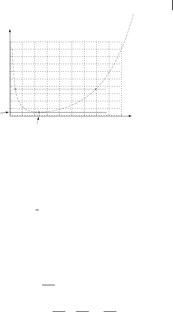
Defining the function G(v)by
G(v) ≡
cosh v
v
, (9.7.44)
G(v) is plotted in Figure 9.4.
If the geometry of the problem is such that
RL > 1.5089,
then there exist two candidates for the solution at v = v
<
and v = v
>
,where
0 <v
<
< 1.1997 <v
>
,
9.7 The Second Variation 341
0.0 0.5 1.0 1.5 2.0 2.5 3.0 3.5 4.0 4.5
1
2
1.5089
1.1997
3
4
5
6
7
8
9
10
11
G
(
v
)
v
v
<
v
>
Fig. 9.4 Plot of G(v).
and if
RL < 1.5089,
then there exists no solution.Ifthegeometryissuchthat
RL = 1.5089,
then there exists one candidate for the solution at
v
<
= v
>
= v =
L
α
= 1.1997.
We apply two tests for the minimum.
Legendre test:
f
y
y
= y(1 + y
2
)
3/2
= R > 0,
thus passing the Legendre test.
Jacobi test:Since
y(x, α, β) = α cosh(
x − β
α
),
we have
u
1
(x) = ∂y∂α = cosh(
x − β
α
) − (
x − β
α
)sinh(
x − β
α
),
342 9 Calculus of Variations: Fundamentals
~
v
1.1997
~
v
1
~
v
1
~
v
2
~
v
2
~
v
ξ
~
v
ξ
F
(
v
)
~
Fig. 9.5 Plot of F( ˜v).
and
u
2
(x) =−∂y∂β = sinh(
x − β
α
),
where the minus sign for u
2
(x) does not matter. We construct a solution U(x)
which vanishes at x = x
1
,
U(x) = (cosh ˜v −˜v sinh ˜v)sinh ˜v
1
− sinh ˜v(cosh ˜v
1
−˜v
1
sinh ˜v
1
),
where
˜v ≡
x − β
α
, ˜v
1
≡
x
1
− β
α
.
Then we have
U(x)(sinh ˜v sinh ˜v
1
) = (coth ˜v −˜v) − (coth ˜v
1
−˜v
1
).
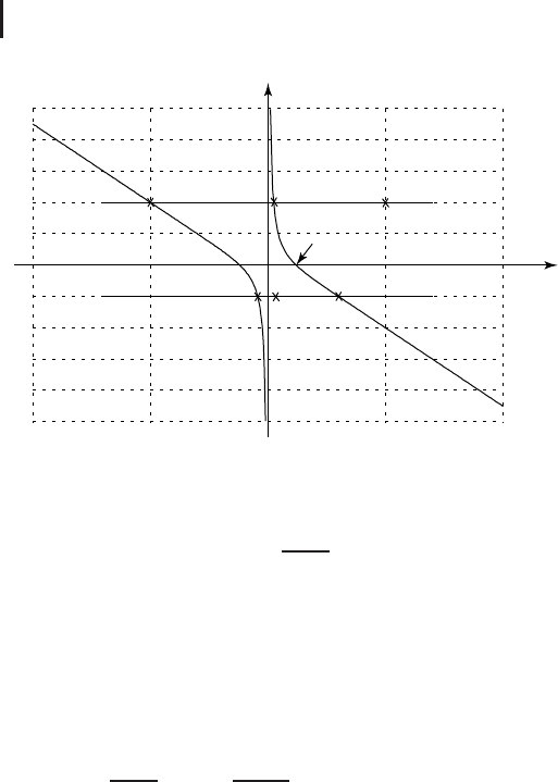
Defining the function F( ˜v)by
F( ˜v) ≡ coth ˜v −˜v, (9.7.45)
F( ˜v) is plotted in Figure 9.5.
We have
U(x)(sinh ˜v sinh ˜v
1
) = F( ˜v) − F( ˜v
1
).
Note that F( ˜v) is an odd function of ˜v,
F(−˜v) =−F( ˜v).

9.7 The Second Variation 343
We set
˜v
1
≡−
L
α
, ˜v
2
≡+
L
α
, ˜v
ξ
≡
ξ
α
,
where
β = 0,
is used. The equation,
U(ξ ) = 0, ξ = x
1
,
which determines the conjugate point ξ , is equivalent to the following equation:
F( ˜v
ξ
) = F( ˜v
1
), ˜v
ξ
=˜v
1
.
If
F( ˜v
1
) > 0, (9.7.46)
then,fromFigure9.5,wehave
˜v
1
< ˜v
ξ
< ˜v
2
,
thus failing the Jacobi test. If, on the other hand,
F( ˜v
1
) < 0, (9.7.47)
then,fromFigure9.5,wehave
˜v
1
< ˜v
2
< ˜v
ξ
,
thus passing the Jacobi test. The dividing line
F( ˜v
1
) = 0
corresponds to
˜v
1
< ˜v
2
=˜v
ξ
,
and thus we have one solution at
˜v
2
=−˜v
1
=
L
α
= 1.1997.

344 9 Calculus of Variations: Fundamentals
Having derived the particular statements of the Jacobi test as applied to this example,
Eqs. (9.7.46) and (9.7.47), we now test which of the two candidates for the solution,
v = v
<
and v = v
>
, is actually the minimizing solution. Two functions, G(v)and
F(v), defined by Eqs. (9.7.44) and (9.7.45), are related to each other through
d
dv
G(v) =−(
sinh v
v
2
)F(v). (9.7.48)
At v = v
<
,weknowfromFigure9.4that
d
dv
G(v
<
) < 0,
which implies
F(−v
<
) =−F(v
<
) < 0,
so that one candidate, v = v
<
, passes the Jacobi test and is the solution, whereas at
v = v
>
,weknowfromFigure9.4that
d
dv
G(v
>
) > 0,
which implies
F(−v
>
) =−F(v
>
) > 0,
so that the other candidate, v = v
>
, fails the Jacobi test and is not the solution.
When two candidates, v = v
<
and v = v
>
, coalesce to a single point,
v = 1.1997,
where the first derivative of G(v) vanishes, i.e.,
d
dv
G(v) = 0,
v
<
= v
>
= 1.1997 is the solution.
We now consider a strong variation and the condition for the strong minimum.In
the strong variation, since the varied derivatives behave very differently from the
original derivatives, we cannot expand the integral I inTaylorseries.Instead,we
consider the Weierstrass E function defined by
E(x, y
0
, y
0
, p) ≡ f (x, y
0
, p) −
f (x, y
0
, y
0
) + (p − y
0
)f
y
(x, y
0
, y
0
)
. (9.7.49)

9.8 Weierstrass–Erdmann Corner Relation 345
Necessary and sufficient conditions for the strong minimum are given by
Necessary condition Sufficient condition
(1) f
y
y
(x, y
0
, y
0
) ≥ 0,
where y
0
is the solution
of the Euler equation
(1) f
y
y
(x, y, p) > 0,
for every (x, y)closeto(x, y
0
),
and every finite p
(2) ξ ≥ x
2
(2) ξ>x
2
(3) E(x, y
0
, y
0
, p) ≥ 0,
for all finite p,andx ∈ [x
1
, x
2
].
(9.7.50)
We remark that if
p ∼ y
0
,
then we have
E ∼ f
y
y
(x, y
0
, y
0
)
(p − y
0
)
2
2!
,
just like the mean value theorem of ordinary function f (x), which is given by
f (x) − f (x
0
) − f
(x
0
) =
(x − x
0
)
2
2!
f
(x
0
+ λ(x − x
0
)), 0 <λ<1.
9.8
Weierstrass–Erdmann Corner Relation
In this section, we consider the variational problem with the solutions which are
the piecewise continuous functions with corners, i.e., the function itself is continuous,
but the derivative is not. We maximize the integral
I =
x
2
x
1
f (x, y, y
)dx. (9.8.1)
We put a point of corner at x = a. We write the solution for x ≤ a,asy(x)and,for
x > a,asY(x). Then we have from the continuity of the solution,
y(a) = Y(a). (9.8.2)
Now consider the variation of y(x)andY(x) of the following forms:
y(x) → y(x) + εν(x), Y(x) → Y(x) + εV(x), (9.8.3a)
and
y
(x) → y
(x) + εν
(x), Y
(x) → Y
(x) + εV
(x). (9.8.3b)
346 9 Calculus of Variations: Fundamentals
Under these variations , we require I to be stationary,
I =
a
x
1
f (x, y, y
)dx +
x
2
a
f (x, Y, Y
)dx. (9.8.4)
First, we consider the variation problem with the point of the discontinuity of
the derivative at x = a fixed. We have
ν(a) = V(a). (9.8.5)
Performing the above variations, we have
δI =
a
x
1
f
y
εν + f
y
εν
dx +
x
2
a
f
Y
εV +f
Y
εV
dx
= f
y
εν
x=a
x=x
1
+
a
x
1
εν
f
y
−
d
dx
f
y
dx
+ f
Y
εV
x=x
2
x=a
+
x
2
a
εV
f
Y
−
d
dx
f
Y
dx = 0.
If the variations vanish at both ends (x = x
1
and x = x
2
), i.e.,
ν(x
1
) = V(x
2
) = 0, (9.8.6)
we have the following equations:
f
y
−
d
dx
f
y
= 0, x ∈ [x
1
, x
2
] (9.8.7)
and
f
y
x=a
−
= f
Y
x=a
+
,
namely
f
y
is continuous at x = a. (9.8.8)
Next, we consider the variation problem with the point of the discontinuity of
the derivative at x = a varied, i.e.,
a → a + a. (9.8.9)