Mavko G., Mukerji T., Dvorkin J. The Rock Physics Handbook

Подождите немного. Документ загружается.

However, this result is inadequate for small aspect ratio cracks with soft-fluid

saturation, such as when the parameter o ¼K

fluid

/aK is of the order of 1. Then the

appropriate equations given by O’Connell and Budiansky are



¼ 1 

ð1  v

2

ð1  2v



¼ 1 

ð1  v



Þ D þ

ð2  v





e ¼

ðv  v



ð1  v



ð2  v



Dð1 þ 3vÞð2  v



Þ2ð1  2vÞ



D ¼ 1 þ

ð1  v

2

ð1  2v





1

Wu’s self-consistent modulus estimates for two-phase composites may be

expressed as (m ¼matrix, i ¼inclusion)



¼ K

þ x

ðK

 K

ÞP

i



¼ m

þ x

ðm

 m

ÞQ

i

Berryman (1980b, 1995) gives a more general form of the self-consistent approxima-

tions for N-phase composites:

i¼1

ðK

 K



ÞP

i

¼ 0

i¼1

ðm

 m



ÞQ

i

¼ 0

where i refers to the ith material, x

is its volume fraction, P and Q are geometric

factors given in Table 4.8.1, and the superscript *i on P and Q indicates that the

Table 4.8.1 Coefficients P and Q for some specific shapes. The subscripts

m and i refer to the background and inclusion materials (from Berryman 1995).

Inclusion shape P

Spheres

þ z

Needles

þ m

þ 2

þ g

þ m

Disks

þ z

Penny cracks

þ pab

1 þ

þ paðm

þ 2b

þ 2

ðm

þ m

þ pab

Notes:

b ¼ m

ð3KþmÞ

ð3Kþ4mÞ

; g ¼ m

ð3KþmÞ

ð3Kþ7mÞ

; z ¼

ð9Kþ8mÞ

ðKþ2mÞ

, a ¼ crack aspect ratio, a disk is a crack of zero thickness.

187 4.8 Self-consistent approximations of effective moduli

factors are for an inclusion of material i in a background medium with self-consistent

effective moduli K



and m



. The summation is over all phases, including minerals

and pores. These equations are coupled and must be solved by simultaneous iteration.

Although Berryman’s self-consistent method does not converge for fluid disks

¼0), the formulas for penny-shaped fluid-filled cracks are generally not singular

and converge rapidly. However, his estimates for needles, disks, and penny cracks

should be used cautiously for fluid-saturated composite materials.

Dry cavities can be modeled by setting the inclusion moduli to zero. Fluid-

saturated cavities are simulated by setting the inclusion shear modulus to zero.

Caution

Because the cavities are isolated with respect to flow, this approach simulates

very-high-frequency saturated rock behavior appropriate to ultrasonic laboratory

conditions. At low frequencies, when there is time for wave-induced pore-pressure

increments to flow and equilibrate, it is better to find the effective moduli for dry

cavities and then saturate them with the Gassmann low-frequency relations. This

should not be confused with the tendency to term this approach a low-frequency

theory, for crack dimensions are assumed to be much smaller than a wavelength.

Calculate the self-consistent effective bulk and shear moduli, K



, and m



, for a

water-saturated rock consisting of spherical quartz grains (aspect ratio a ¼1) and

total porosity 0.3. The pore space consists of spherical pores (a ¼1) and thin,

penny-shaped cracks (a ¼10

–2

). The thin cracks have a porosity of 0.01, whereas

the remaining porosity (0.29) is made up of the spherical pores.

The total number of phases, N,is3.

(quartz) ¼37 GPa, m

(quartz) ¼44 GPa,

¼1, x

(volume fraction) ¼0.7

(water, spherical pores) ¼2.25 GPa,

(water, spherical pores) ¼0 GPa,

(spherical pores) ¼1, x

(volume fraction) ¼0.29

(water, thin cracks) ¼2.25 GPa,

(water, thin cracks) ¼0 GPa,

(thin cracks) ¼10

2

, x

(volume fraction) ¼0.01

The coupled equations for K



and m



are

ðK

 K



ÞP

1

þ x

ðK

 K



ÞP

2

þ x

ðK

 K



ÞP

3

¼ 0

ðm

 m



ÞQ

1

þ x

ðm

 m



ÞQ

2

þ x

ðm

 m



ÞQ

3

¼ 0

The P’s and Q’s are obtained from Table 4.8.1 or from the more general equation

for ellipsoids of arbitrary aspect ratio. In the equations for P and Q, K

and m

are

188 Effective elastic media: bounds and mixing laws

replaced everywhere by K



and m



, respectively. The coupled equations are

solved iteratively, starting from some initial guess for K



and m



. The Voigt

average may be taken as the starting point. The converged solutions (known as the

fixed points of the coupled equations) are K



¼16.8 GPa and m



¼11.6 GPa.

The coefficients P and Q for ellipsoidal inclusions of arbitrary aspect ratio are

given by

P ¼

iijj

Q ¼

ijij



iijj



where the tensor T

ijkl

relates the uniform far-field strain field to the strain within the

ellipsoidal inclusion (Wu, 1966). Berryman (1980b) gives the pertinent scalars

required for computing P and Q as

iijj

ijij



iijj

þ F

 F

where

¼ 1 þ A

ðf þ yÞR

f þ

y 



¼ 1 þ A 1 þ

ðf þ yÞ

Rð3f þ 5yÞ



þ Bð3  4RÞ

AðA þ 3BÞð3  4RÞ½f þ y  Rðf  y þ 2y

Þ

¼ 1 þ A 1  f þ



þ Rðf þ yÞ



¼ 1 þ

A½f þ 3y  Rðf  yÞ

¼ A f þ Rfþ y 



þ Byð3  4RÞ

¼ 1 þ A½1 þ f  Rðf þ yÞ þ Bð1  yÞð3  4RÞ

¼ 2 þ

A½3f þ 9y  Rð3f þ 5yÞ þ Byð3  4RÞ

¼ A½1  2R þ

f ðR  1Þþ

yð5R  3Þþ Bð1  yÞð3  4RÞ

¼ A½ðR  1Þf  RyþByð3 4RÞ

189 4.8 Self-consistent approximations of effective moduli

with A, B, and R given by

A ¼ m

 1

B ¼





and

R ¼

ð1  2v

2ð1  v

The functions y and f are given by

y ¼

ða

 1Þ

3=2

aða

 1Þ

1=2

 cosh

1

ð1  a

3=2

cos

1

a  að1  a

1=2

for prolate and oblate spheroids, respectively, and

f ¼

1  a

ð3y  2Þ

Note that a < 1 for oblate spheroids and a > 1 for prolate spheroids.

Assumptions and limitations

The approach described in this section has the following presuppositions:



idealized ellipsoidal inclusion shapes;



isotropic, linear, elastic media; and



cracks are isolated with respect to fluid flow. Pore pressures are unequilibrated and

adiabatic, which is appropriate for high-frequency laboratory conditions. For low-

frequency field situations, use dry inclusions and then saturate by using Gassmann

relations. This should not be confused with the tendency to term this approach a

low-frequency theory, for crack dimensions are assumed to be much smaller than

a wavelength.

4.9 Differential effective medium model

Synopsis

The differential effective medium (DEM) theory models two-phase composites by

incrementally adding inclusions of one phase (phase 2) to the matrix phase (Cleary

et al., 1980; Norris, 1985; Zimmerman, 1991a). The matrix begins as phase 1 (when

the concentration of phase 2 is zero) and is changed at each step as a new increment

of phase 2 material is added. The process is continued until the desired proportion of

190 Effective elastic media: bounds and mixing laws

the constituents is reached. The DEM formulation does not treat each constituent

symmetrically. There is a preferred matrix or host material, and the effective moduli

depend on the construction path taken to reach the final composite. Starting with

material 1 as the host and incrementally adding inclusions of material 2 will not, in

general, lead to the same effective properties as starting with phase 2 as the host.

For multiple inclusion shapes or multiple constituents, the effective moduli depend

not only on the final volume fractions of the constituents but also on the order in

which the incremental additions are made. The process of incrementally adding

inclusions to the matrix is really a thought experiment and should not be taken to

provide an accurate description of the true evolution of rock porosity in nature.

The coupled system of ordinary differential equations for the effective bulk and

shear moduli, K* and m*, respectively, are (Berryman, 1992b)

ð1  yÞ

½K



ðyÞ ¼ ðK

 K



ÞP

ð2Þ

ðyÞ

ð1  yÞ

½m



ðyÞ ¼ ðm

 m



ÞQ

ð2Þ

ðyÞ

with initial conditions K*(0) ¼K

and m*(0) ¼m

, where K

and m

are the bulk and

shear moduli of the intial host material (phase 1), K

and m

are the bulk and shear

moduli of the incrementally added inclusions (phase 2), and y is the concentration of

phase 2.

For fluid inclusions and voids, y equals the porosity, f. The terms P and Q are

geometric factors given in Table 4.9.1, and the superscript *2 on P and Q indicates that

the factors are for an inclusion of material 2 in a background medium with effective

moduli K*andm*. Dry cavities can be modeled by setting the inclusion moduli to zero.

Fluid-saturated cavities are simulated by setting the inclusion shear modulus to zero.

Table 4.9.1 Coefficients P and Q for some specific shapes. The subscripts m and i

refer to the background and inclusion materials (from Berryman 1995).

Inclusion shape P

Spheres

þ z

Needles

þ m

þ 2

þ g

þ m

Disks

þ z

Penny cracks

þ pab

1 þ

þ paðm

þ 2b

þ 2

ðm

þ m

þ pab

Notes:

b ¼ m

ð3KþmÞ

ð3Kþ4mÞ

; g ¼ m

ð3KþmÞ

ð3Kþ7mÞ

; z ¼

ð9Kþ8mÞ

ðKþ2mÞ

, a ¼ crack aspect ratio, a disk is a crack of zero thickness.

191 4.9 Differential effective medium model

Caution

Because the cavities are isolated with respect to flow, this approach simulates very-

high-frequency saturated rock behavior appropriate to ultrasonic laboratory condi-

tions. At low frequencies, when there is time for wave-induced pore-pressure

increments to flow and equilibrate, it is better to find the effective moduli for

dry cavities and then saturate them with the Gassmann low-frequency relations. This

should not be confused with the tendency to term this approach a low-frequency

theory, for inclusion dimensions are assumed to be much smaller than a wavelength.

The P and Q for ellipsoidal inclusions with arbitrary aspect ratio are the same as

given in Section 4.8 for the self-consistent methods, and are repeated in Table 4.9.1.

Norris et al. (1985) have shown that the DEM is realizable and therefore is always

consistent with the Hashin–Shtrikman upper and lower bounds.

The DEM equations as given above (Norris, 1985; Zimmerman, 1991b; Berryman

et al., 1992) assume that, as each new inclusion (or pore) is introduced, it displaces on

average either the host matrix material or the inclusion material, with probabilities

(1 – y) and y, respectively. A slightly different derivation by Zimmerman (1984)

(superseded by Zimmerman (1991a)) assumed that when a new inclusion is intro-

duced, it always displaces the host material alone. This leads to similar differential

equations with dy/(1 – y) replaced by dy. The effective moduli predicted by this

version of DEM are always slightly stiffer (for the same inclusion geometry and

concentration) than the DEM equations given above. They both predict the same first-

order terms in y but begin to diverge at concentrations above 10%. The dependence of

effective moduli on concentration goes as e

2y

¼ð1  2y þ 2y

Þfor the version

without (1 y), whereas it behaves as (1 y)

¼(1 2y þy

) for the version with

(1  y). Including the (1 y) term makes the results of Zimmerman (1991a) consistent

with the Hashin–Shtrikman bounds. In general, for a fixed inclusion geometry and

porosity, the Kuster–Tokso

z effective moduli are stiffer than the DEM predictions,

which in turn are stiffer than the Berryman self-consistent effective moduli.

An important conceptual difference between the DEM and self-consistent schemes

for calculating effective moduli of composites is that the DEM scheme identifies one

of the constituents as a host or matrix material in which inclusions of the other

constituent(s) are embedded, whereas the self-consistent scheme does not identify any

specific host material but treats the composite as an aggregate of all the constituents.

Modified DEM with critical porosity constraints

In the usual DEM model, starting from a solid initial host, a porous material stays

intact at all porosities and falls apart only at the very end when y ¼1 (100% porosity).

This is because the solid host remains connected, and therefore load bearing.

Although DEM is a good model for materials such as glass foam (Berge et al.,

1993) and oceanic basalts (Berge et al., 1992), most reservoir rocks fall apart at

192 Effective elastic media: bounds and mixing laws

a critical porosity, f

, significantly less than 1.0 and are not represented very well by

the conventional DEM theory. The modified DEM model (Mukerji et al., 1995a)

incorporates percolation behavior at any desired f

by redefining the phase 2 end-

member. The inclusions are now no longer made up of pure fluid (the original phase 2

material) but are composite inclusions of the critical phase at f

with elastic moduli

, m

). With this definition, y denotes the concentration of the critical phase in the

matrix. The total porosity is given by f ¼yf

The computations are implemented by replacing (K

, m

) with (K

, m

) everywhere

in the equations. Integrating along the reverse path, from f ¼f

to f ¼0 gives lower

moduli, for now the softer critical phase is the matrix. The moduli of the critical phase

may be taken as the Reuss average value at f

of the pure end-member moduli.

Because the critical phase consists of grains just barely touching each other, better

estimates of K

and m

may be obtained from measurements on loose sands, or from

models of granular material. For porosities greater than f

, the material is a suspen-

sion and is best characterized by the Reuss average (or Wood’s equation).

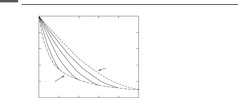
Figure 4.9.1 shows normalized bulk-modulus curves for the conventional

DEM theory (percolation at f ¼1) and for the modified DEM (percolation at

< 1) for a range of f

values. When f

¼1, the modified DEM coincides with

the conventional DEM curve. The shapes of the inclusions were taken to be spheres.

The path was from 0 to f

, and (K

, m

) were taken as the Reuss-average values at f

For this choice of (K

, m

), estimates along the reversed path coincide with the Reuss

curve.

Uses

The purpose of the differential effective-medium model is to estimate the effective

elastic moduli of a rock in terms of its constituents and pore space.

0.2

0.4

0.6

0.8

0 0.2 0.4 0.6 0.8 1

Bulk moduli (normalized)

Porosity

0.4

0.6

0.8

1.0

Reuss

= 0.2

DEM

Figure 4.9.1 Normalized bulk-modulus curves for the conventional DEM theory (percolation

at f ¼ 1) and for the modified DEM (percolation at f

< 1) for a range of f

values.

193 4.9 Differential effective medium model

Assumptions and limitations

The following assumptions and limitations apply to the differential effective-medium

model:



the rock is isotropic, linear, and elastic;



the process of incrementally adding inclusions to the matrix is a thought experiment

and should not be taken to provide an accurate description of the true evolution of

rock porosity in nature;



idealized ellipsoidal inclusion shapes are assumed; and



cracks are isolated with respect to fluid flow. Pore pressures are unequilibrated and

adiabatic. The model is appropriate for high-frequency laboratory conditions. For low-

frequency field situations, use dry inclusions and then saturate using Gassmann relations.

This should not be confused with the tendency to term this approach a low-frequency

theory, for crack dimensions are assumed to be much smaller than a wavelength.

4.10 Hudson’s model for cracked media

Synopsis

Hudson’s model is based on a scattering-theory analysis of the mean wavefield in an

elastic solid with thin, penny-shaped ellipsoidal cracks or inclusions (Hudson, 1980,

1981). The effective moduli c

eff

are given as

eff

¼ c

þ c

where c

are the isotropic background moduli, and c

, c

are the first- and second-

order corrections, respectively. (See Section 2.2 on anisotropy for the two-index

notation of elastic moduli. Note also that Hudson uses a slightly different definition

and that there is an extra factor of 2 in his c

, c

, and c

. This makes the equations

given in his paper for c

and c

slightly different from those given below, which are

consistent with the more standard notation described in Section 2.2 on anisotropy.)

For a single crack set with crack normals aligned along the 3-axis, the cracked

media show transverse isotropic symmetry, and the corrections are

¼

lðl þ 2mÞ

¼

ðl þ 2mÞ

¼meU

¼0

194 Effective elastic media: bounds and mixing laws

and (superscripts on c

denote second order, not quantities squared)

ðl þ 2mÞ

ðeU

lðeU

ðl þ 2mÞðeU

mð3l þ 8mÞ

l þ 2m

ðeU

¼ 0

where

q ¼ 15

þ 28

e ¼

3

4pa

¼ crack density

The isotropic background elastic moduli are l and m,anda and a are the crack radius

and aspect ratio, respectively. The corrections c

and c

obey the usual symmetry

properties for transverse isotropy or hexagonal symmetry (see Section 2.2 on anisotropy).

Caution

The second-order expansion is not a uniformly converging series and predicts

increasing moduli with crack density beyond the formal limit (Cheng, 1993).

Better results will be obtained by using just the first-order correction rather than

inappropriately using the second-order correction. Cheng gives a new expansion

based on the Pade

approximation, which avoids this problem.

The terms U

and U

depend on the crack conditions. For dry cracks

16ðl þ 2mÞ

3ð3l þ 4mÞ

4ðl þ 2mÞ

3ðl þ mÞ

For “weak” inclusions (i.e., when ma=ðK

Þ is of the order of 1 and is not small

enough to be neglected)

16ðl þ 2mÞ

3ð3l þ 4mÞ

ð1 þ MÞ

4ðl þ 2mÞ

3ðl þ mÞ

ð1 þ k Þ

195 4.10 Hudson’s model for cracked media

where

M ¼

pam

ðl þ 2mÞ

ð3l þ 4mÞ

k ¼

ðK

Þðl þ 2mÞ

pamðl þ mÞ

where K

and m

are the bulk and shear modulus of the inclusion material. The criteria

for an inclusion to be “weak” depend on its shape or aspect ratio a as well as on the

relative moduli of the inclusion and matrix material. Dry cavities can be modeled by

setting the inclusion moduli to zero. Fluid-saturated cavities are simulated by setting

the inclusion shear modulus to zero.

Caution

Because the cavities are isolated with respect to flow, this approach simulates very-

high-frequency behavior appropriate to ultrasonic laboratory conditions. At low

frequencies, when there is time for wave-induced pore-pressure increments to flow

and equilibrate, it is better to find the effective moduli for dry cavities and then

saturate them with the Brown and Korringa low-frequency relations (Section 6.5).

This should not be confused with the tendency to term this approach a low-frequency

theory, for crack dimensions are assumed to be much smaller than a wavelength.

Hudson also gives expressions for infinitely thin, fluid-filled cracks:

16ðl þ2 mÞ

3ð3l þ4 mÞ

¼ 0

These assume no discontinuity in the normal component of crack displacements and

therefore predict no change in the compressional modulus with saturation. There is,

however, a shear displacement discontinuity and a resulting effect on shear stiffness.

This case should be used with care.

The first-order changes l

and m

in the isotropic elastic moduli l and m of a

material containing randomly oriented inclusions are given by

¼

eð3U

þ 2U

þ 2m

¼

ð3l þ 2mÞ

These results agree with the self-consistent results of Budiansky and O’Connell (1976).

For two or more crack sets aligned in different directions, corrections for each

crack set are calculated separately in a crack-local coordinate system with the 3-axis

normal to the crack plane and then rotated or transformed back (see Section 1.4 on

coordinate transformations) into the coordinates of c

eff

; finally the results are added to

196 Effective elastic media: bounds and mixing laws