Middleton W.M. (ed.) Reference Data for Engineers: Radio, Electronics, Computer and Communications
Подождите немного. Документ загружается.

10-1
0
REFERENCE
DATA
FOR ENGINEERS
Although the above sensitivity discussion has been
concentrated solely on deviations of the transfer func-
tion
H(s)
caused by component changes, it should be
understood that sensitivity calculations apply to any
network parameter whose value depends
on
variable
circuit components. For example, the center frequency
and the selectivity of
a
bandpass function, or the cutoff
frequency of
a
low-pass filter, depend in general on
several resistors and capacitors and possibly on op-
amp or OTA gain. Any shift in these parameters result-
ing from component variations can be estimated by
calculating the corresponding sensitivities. Similarly,
the precise location of transmission zeros or filter
poles depends, of course,
on
the correct element Val-
ues. Any variations or tolerances in the latter cause
shifts in these critical frequencies and therefore trans-
fer-function errors that can readily be evaluated by
sensitivity calculations. All second- and higher-order
filters discussed in the remaining four sections of this
chapter have been evaluated extensively
as
to their sen-
sitivity performance and
are
recognized
as
the best
designs available. If a different active
RC
filter out of
the numerous topologies presented in the literature
is
to be used, the sensitivities of the contemplated circuit
should be carefully investigated to make sure that the
design will work satisfactorily in practice. It is noted
again that simple postdesign tuning to eliminate fabri-
cation tolerances will in general not suffice because
circuit components cannot be expected to retain their
values under environmental stresses, such as aging or
temperature fluctuations, Thus, low sensitivity is
a
necessary requirement for any circuit. When evaluat-
ing a filter, the reader ought
to
keep in mind that the
sensitivity results presented are valid for
small
changes
in element values because of the linearization
involved in the analysis: Note from Eq. 21 that the
function
HGw,
k)
has been replaced by its slope in the
nominal point
k
=
ko
to estimate changes caused by
varying
k
from
k,
to
ko
+
Ak.
In
particular, this means
that
a
circuit with the desirable property
Sf
=
0
may
not
be entirely independent of the parameter
k;
it only
says that
at
the nominal value
k
=
k,
the slope
dH/dk
is
zero, usually implying
a
quadratic dependence on
k.
Large variations
Ak
can still cause unacceptable per-
formance errors!
It is also emphasized that sensitivity expressions are
usually functions
of
frequency
so
that
the results ought
to
be evaluated in the frequency range of interest (nor-
mally in the passband or at the passband edges) when
different possible designs are compared.
Finally, a last point is worth noting: Sensitivity is
only an intermediate result and by itself can still create
a
misleading picture of circuit performance.
In
the ulti-
mate analysis, what is important is the deviation or
variability
MIH,
Le., by
Eqs.
21 or
24,
the sensitivity
multiplied by the expected component tolerances.
Hence, relatively large sensitivities are acceptable
when the relevant “component” (e.g.,
a
resistor ratio
in
a
thin-film hybrid realization) can be expected
to
be
very accurate and stable. However, when
a
component
varies strongly (e.g., op-amp gain-bandwidth prod-
uct), very low sensitivities must be insisted upon.
FREQUENTLY USED BUILDING
BLOCKS
Active filters are generally constructed by intercon-
necting
a
number of well-understood elementary
building blocks. Understanding the performance of
those blocks enables the designer
to
assemble
a
filter
that works better and more reliably. Thus, in this sec-
tion, the most important functional blocks are being
introduced: the summer, the integrator, the general
impedance converter
(GIC),
the gyrator (which is
a
cir-
cuit that is used
to
simulate an inductor via
a
capaci-
tor), the frequency-dependent negative resistor
(FDNR),
and
a
circuit for realizing
a
first-order voltage
transfer function. A separate section is devoted
to
the
realization of second-order biquadratic transfer func-
tions because of their special importance.
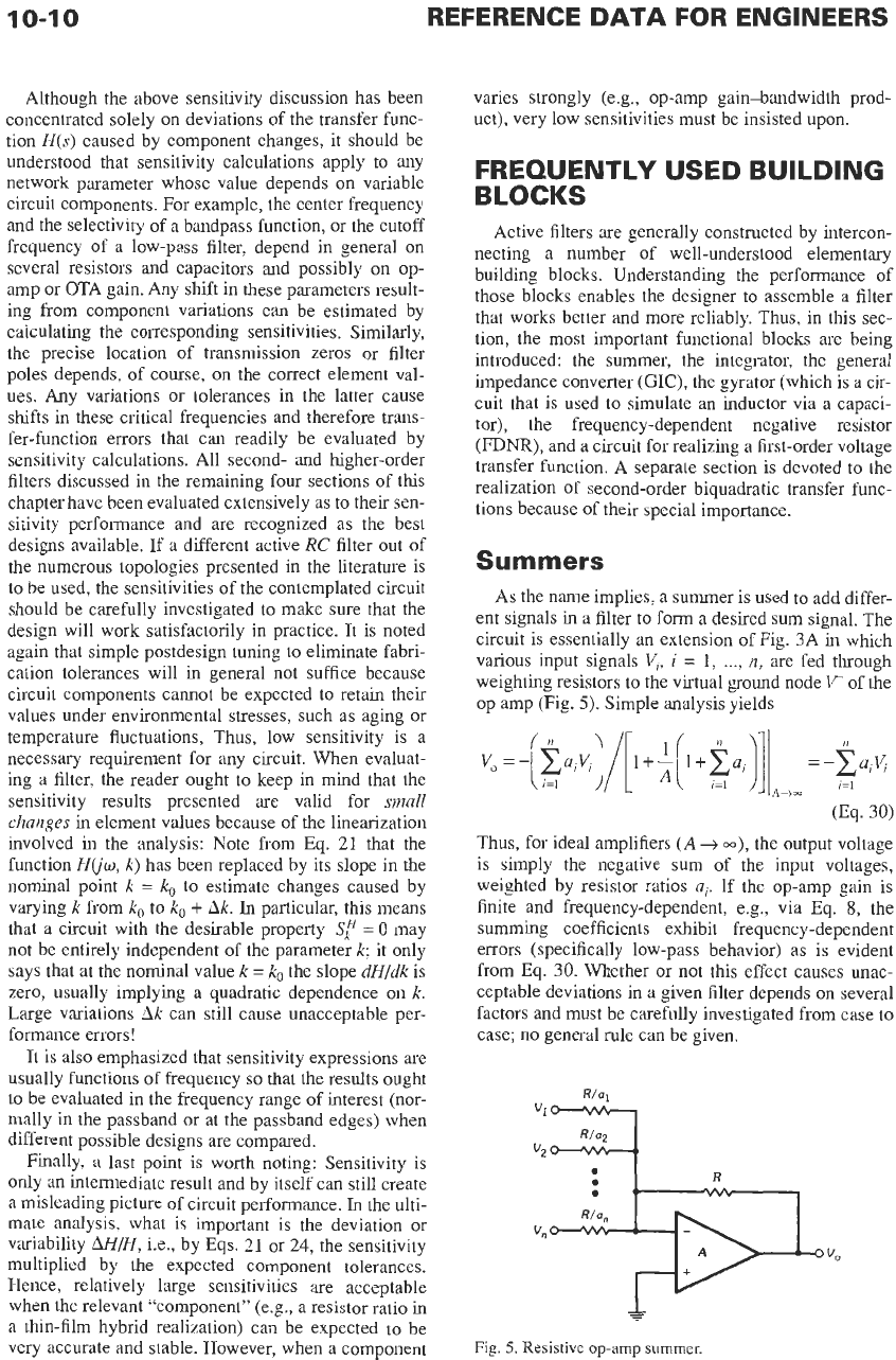
Summers
As
the name implies, a summer is used
to
add differ-
ent signals in
a
filter to form
a
desired sum signal. The
circuit is essentially an extension of Fig. 3A in which
various input signals
V,,
i
=
1,
...,
n,
are fed through
weighting resistors to the virtual ground node
V
of the
op amp (Fig.
5).
Simple analysis yields
(Eq.
30)
Thus, for ideal amplifiers
(A
+
CQ),
the output voltage
is simply the negative sum of the input voltages,
weighted by resistor ratios
ai.
If the op-amp gain is
finite and frequency-dependent, e.g., via Eq.
8,
the
summing coefficients exhibit frequency-dependent
errors (specifically low-pass behavior)
as
is evident
from Eq.
30.
Whether or not this effect causes unac-
ceptable deviations in
a
given filter depends on several
factors and must be carefully investigated from case
to
case; no general rule can be given.
g5
Fig.
5.
Resistive
op-amp
summer.
ACTIVE FILTER DESIGN
10-1
1
In
an OTA design, voltages are converted at each
stage into currents as indicated by Eq.
14.
Current
summing
is performed
automatically
at any circuit
node via Kirchhoff's current law and
so
does not cost
any elements. The designer is advised, therefore, to
construct the circuit such that required summing func-
tions
are
performed with currents rather than voltages.
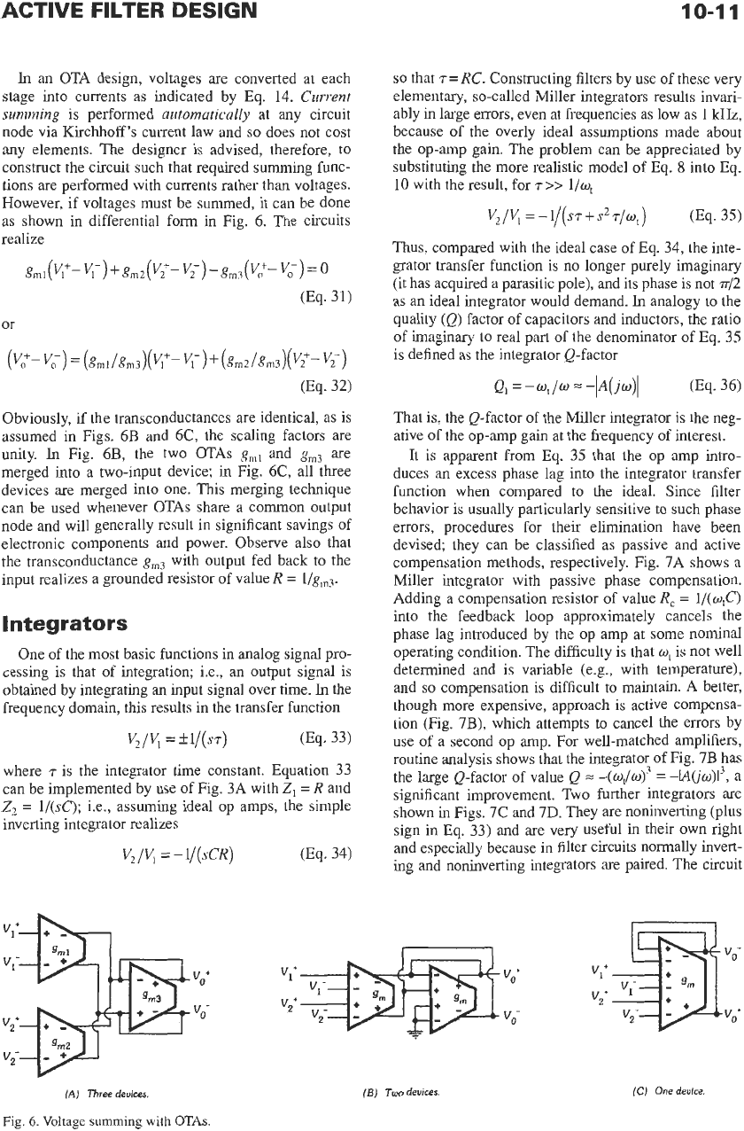
However, if voltages must be summed, it can be done
as shown in differential form in Fig.
6.
The circuits
realize
or
(V;-K)
=
(gml
/gm,)(V,+-
v;)
+
(gm2
/gm,)(V;-vc)
(Eq.
32)
Obviously,
if
the transconductances are identical, as is
assumed in Figs.
6B
and
6C,
the scaling factors are
unity.
In
Fig.
6B,
the two
OTAs
gm,
and
g,,
are
merged into a two-input device; in Fig.
6C,
all three
devices are merged into one. This merging technique
can be used whenever
OTAs
share a common output
node and will generally result in significant savings of
electronic components and power. Observe also that
the transconductance
gm,
with output fed back to the
input realizes a grounded resistor of value
R
=
l/gm3.
In
teg rat0 r
s
One of the most basic functions in analog signal pro-
cessing is that of integration; i.e., an output signal is
obtained by integrating an input signal over time.
In
the
frequency domain, this results in the transfer function
v2/y
=
kl/(ST)
(Eq.
33)
where
r
is the integrator time constant. Equation
33
can be implemented by use of Fig.
3A
with
2,
=
R
and
Z2
=
l/(sC);
i.e., assuming ideal op amps, the simple
inverting integrator realizes
V2
/V,
=
-
1/(
sCR)
0%.
34)
so
that
T
=
RC.
Constructing filters by use of these very
elementary, so-called Miller integrators results invari-
ably in large errors, even at frequencies as low as
1
Wz,
because of the overly ideal assumptions made about
the op-amp gain. The problem can be appreciated by
substituting the more realistic model of Eq.
8
into Eq.
10
with the result, for
7
>>
l/w,
V2/V,
=-1/(m+s2~/wt)
(Eq.
35)
Thus, compared with the ideal case of Eq.
34,
the inte-
grator transfer function is
no
longer purely imaginary
(it has acquired a parasitic pole), and its phase is not
~/2
as an ideal integrator would demand.
In
analogy to the
quality (Q) factor of capacitors and inductors, the ratio
of
imaginary to real part of the denominator of Eq.
35
is defined as the integrator Q-factor
Q,
=-wt/u=-IA(jw)l
(Eq.
36)
That is, the Q-factor of the Miller integrator is the neg-
ative of the op-amp gain at the frequency of interest.
It
is apparent from Eq.
35
that the op amp intro-
duces an excess phase lag into the integrator transfer
function when compared to the ideal. Since filter
behavior is usually particularly sensitive
to
such phase
errors, procedures for their elimination have been
devised; they can be classified as passive and active
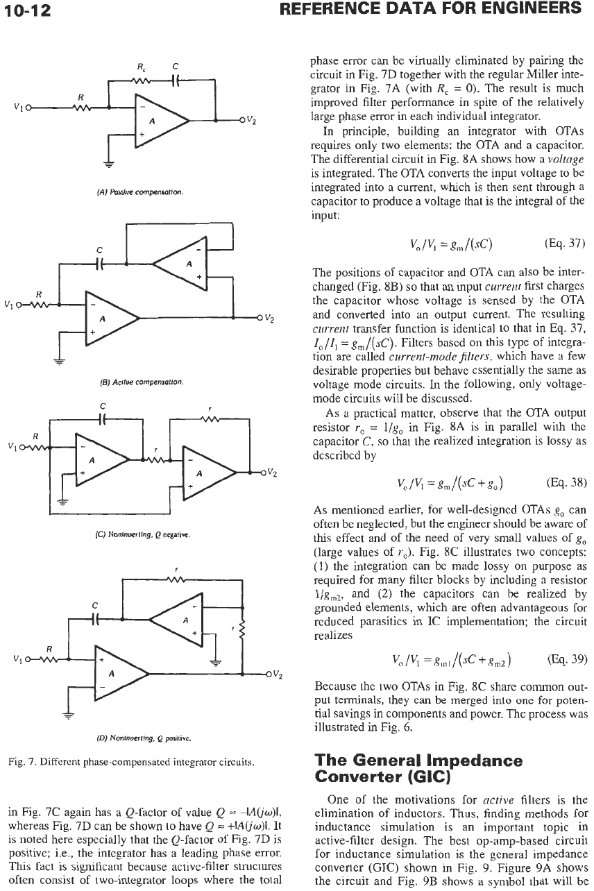
compensation methods, respectively. Fig.
7A
shows a
Miller integrator with passive phase compensation.
Adding a compensation resistor of value
R,
=
l/(wtC)
into the feedback loop approximately cancels the
phase lag introduced by the op amp at some
nominal
operating condition. The difficulty is that
w,
is
not
well
determined and is variable (e.g., with temperature),
and so compensation is difficult to maintain.
A
better,
though more expensive, approach is active compensa-
tion (Fig.
7B),
which attempts to cancel the errors by
use of a second op amp. For well-matched amplifiers,
routine analysis shows that the integrator of Fig.
7B
has
the large Q-factor of value Q
=
-(w,/w)~
=
-H(jw)I3,
a
significant improvement. Two further integrators are
shown in Figs,
7C
and
7D.
They are noninverting (plus
sign in Eq.
33)
and are very useful
in
their
own
right
and especially because
in
filter circuits normally invert-
ing and noninverting integrators
are
paired. The circuit
"l+
"z+
(AJ
Three
devices.
Fig.
6.
Voltage
summing
with
OTAs.
(€3)
Two
devices.
(C)
One
device.
10-1
2
REFERENCE
DATA
FOR ENGINEERS
(A)
Paulve cornpensadon.
(6)
Actlue cornpensetton.
C
~
(C)
Nonlnuertlng,
Q
negative
r
C
I
(D)
Nonlnuertlng,
Q
positive
Fig.
7.
Different phase-compensated integrator circuits.
in Fig.
7C
again has a Q-factor of value Q
=
-!AQw)l,
whereas Fig.
7D
can be shown to have Q
=
+IAQw)l.
It
is noted here especially that the Q-factor
of
Fig.
7D
is
positive; i.e., the integrator has a leading phase error.
This fact is significant because active-filter structures
often consist
of
two-integrator loops where the total
phase error can be virtually eliminated by pairing the
circuit
in
Fig.
7D
together with the regular Miller inte-
grator in Fig.
7A
(with
R,
=
0).
The
result is much
improved filter performance in spite of the relatively
large phase error in each individual integrator.
In
principle, building an integrator with OTAs
requires only two elements: the OTA and a capacitor.
The differential circuit in Fig. 8A shows how a
voltage
is integrated. The OTA converts the input voltage
to
be
integrated into a current, which is then sent through a
capacitor to produce a voltage that is the integral
of
the
input:
The positions of capacitor and OTA can also be inter-
changed (Fig. 8B)
so
that an input
current
first charges
the capacitor whose voltage is sensed by the OTA
and converted into an output current. The resulting
current
transfer function is identical to that in
Eq.
37,
Io/Il
=
g,/(sC).
Filters based
on
this type of integra-
tion are called
current-mode filters,
which have a few
desirable properties but behave essentially the same as
voltage mode circuits.
In
the following, only voltage-
mode circuits will be discussed.
As a practical matter, observe that the OTA output
resistor
r,
= l/g,
in Fig. 8A is in parallel with the
capacitor
C,
so
that the realized integration is lossy as
described by
As
mentioned earlier, for well-designed OTAs
go
can
often be neglected, but the engineer should be aware of
this effect and of
the
need of very small values of
go
(large values
of
Yo).
Fig.
8C
illustrates two concepts:
(1)
the integration can be made lossy
on
purpose as
required for many filter blocks by including a resistor
l/gm2,
and
(2)
the capacitors can be realized by
grounded elements, which
are
often advantageous for
reduced parasitics in
IC
implementation; the circuit
realizes
Because the two OTAs
in
Fig.
8C
share common out-
put
terminals, they can be merged into one for poten-
tial savings in components and power. The process was
illustrated in Fig.
6.
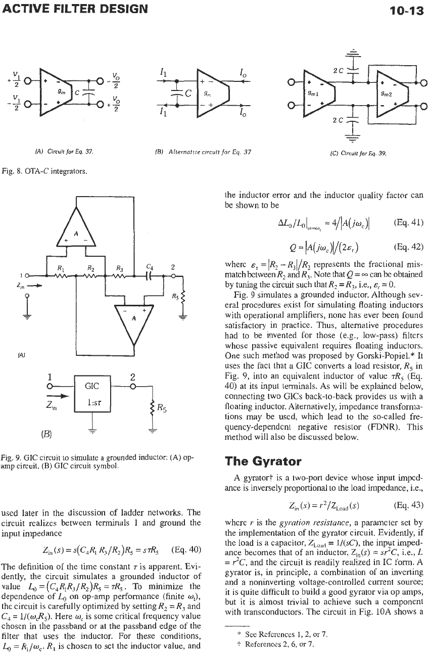
The General Impedance
Converter (GIC)
One of the motivations for
active
filters is the
elimination of inductors. Thus, finding methods for
inductance simulation is an important topic in
active-filter design. The best op-amp-based circuit
for inductance simulation is the general impedance
converter
(GIC)
shown
in
Fig.
9.
Figure 9A shows
the circuit and Fig.
9B
shows a symbol that will be
ACTIVE FILTER DESIGN
10-1
3
-
-
IO
IO
-
-
(A)
Circuit
for
Eq.
37.
(BJ
Alternative
circuit
for
Eq.
37
(CJ Circuit
for
Eq.
39
Fig.
8.
OTA-C
integrators.
fAJ
U
1:sz
Zin
'OR5
Fig.
9.
GIC
circuit
to
simulate
a
grounded inductor:
(A)
op-
amp
circuit,
(B)
GIC
circuit
symbol.
used later in the discussion of ladder networks. The
circuit realizes between terminals
1
and ground the
input impedance
Zh(s)
=
s(C4Rl
R3/R,)R5
=
srR5
(Eq.
40)
The definition
of
the time constant
r
is apparent. Evi-
dently, the circuit simulates a grounded inductor of
value
Lo
=
(C4RlR3/R2)R5
=
rR5.
To
minimize the
dependence of
Lo
on op-amp performance (finite
wJ,
the
circuit is carefully optimized by setting
R,
=
R,
and
C,
=
l/(o&).
Here
w,
is some critical frequency value
chosen in the passband or at the passband edge of the
filter that uses the inductor. For these conditions,
Lo
=
Rl/wc.
R,
is
chosen
to
set the inductor value, and
the inductor error and the inductor quality factor can
be shown to be
where
E,
=
1R2
-
R,I/R,
represents the fractional mis-
match between
R,
and
R,.
Note
that Q
=
m
can be obtained
by tuning the circuit such that
R2
=
R,,
i.e.,
E,
=
0.
Fig.
9
simulates a grounded inductor. Although sev-
eral procedures exist for simulating floating inductors
with operational amplifiers, none has ever been found
satisfactory in practice. Thus, alternative procedures
had to be invented for those (e.g., low-pass) filters
whose passive equivalent requires floating inductors.
One such method was proposed by Gorski-Popiel.* It
uses
the
fact that a GIC converts a load resistor,
R,
in
Fig.
9,
into an equivalent inductor of value
rR5
(Eq.
40)
at its input terminals. As will be explained below,
connecting two GICs back-to-back provides us with a
floating inductor. Alternatively, impedance transforma-
tions may be used, which lead to the so-called fre-
quency-dependent negative resistor
(FDNR).
This
method will also be discussed below.
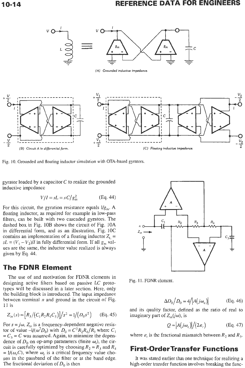
The
Gyrator
A gyrator? is a two-port device whose input imped-
ance is inversely proportional to
the
load impedance, i.e.,
where
Y
is the
gyration resistance,
a parameter set by
the implementation of the gyrator circuit. Evidently, if
the load
is
a capacitor,
ZLoad
=
l/(sC),
the input imped-
ance becomes that of
an
inductor,
Z&)
=
sr2C,
Le.,
L
=
r2C,
and the circuit is readily realized
in
IC form.
A
gyrator is,
in
principle, a combination
of
an inverting
and a noninverting voltage-controlled current source;
it is quite difficult to build
a
good gyrator via op amps,
but it is almost trivial to achieve such a component
with transconductors. The circuit in Fig. 10A shows a
*
See
References
1,
2,
or
7.
t
References
2,
6,
or
7.
10-1
4
REFERENCE DATA FOR ENGINEERS
V
(AJ
Grounded inductive impedance.
I
I
I
I
I
+-
-+
I
I
I
I
I
__
I
___________________
I
2
(BJ
Circuit
A
in dijferentiolform.
L
2
(CJ
Floating inductive impdance.
Fig.
10.
Grounded and floating inductor simulation with OTA-based gyrators.
gyrator loaded by a capacitor C to realize the grounded
inductive impedance
For this circuit, the gyration resistance equals l/g,. A
floating inductor, as required for example in low-pass
filters, can be built with two cascaded gyrators. The
dashed box in Fig.
10B
shows the circuit of Fig. 10A
in
differential form, and as
an
illustration, Fig.
IOC
contains an implementation of a floating inductor
Z,
=
SL
=
(V,
-
V2)/I
in fully differential form. If
all
g,
val-
ues are the same, the inductor value realized is always
given by
Eq.
44.
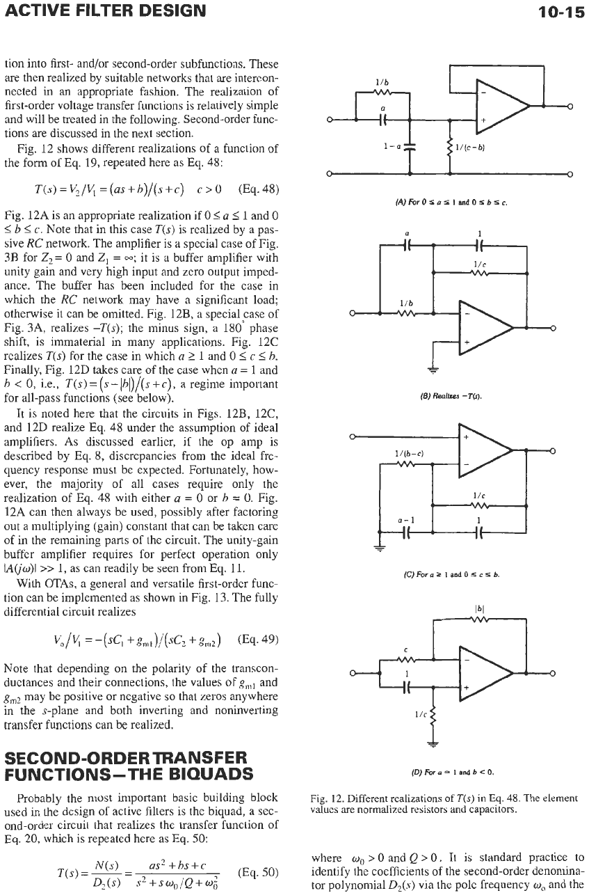
The FDNR Element
The use of and motivation for FDNR elements in
designing active filters based on passive
LC
proto-
types will be discussed in a later section. Here, only
the building block is introduced. The input impedance
between terminal
n
and ground in the circuit of Fig.
11
is
For
s
=
jw,
Zi,
is a frequency-dependent negative resis-
tor of value -l/(w2Do) with Do
=
C2R2R4/R,
where
C,
=
C,
=
C
was assumed. Again, to minimize the depen-
dence
of
Do on op-amp parameters (finite
q),
the cir-
cuit is carefully optimized by choosing
R,
=
R,
and
R,
=
l/(w,C), where
w,
is a critical frequency value cho-
sen in the passband of the filter
or
at the band edge.
The fractional deviation of Do is then
RA
Fig.
11.
FDNR element.
mo/~o
=
4/l4jwC)l
(Eq.
46)
and its quality factor, defined as the ratio of real to
Q
=
IA(jw,
)(/(2~,
)
(Eq.
47)
where
C~
is the fractional mismatch between
R2
and
R,.
First-OrderTransfer Functions
It was stated earlier that one technique for realizing a
high-order transfer function involves breaking the fmc-
ACTIVE FILTER
DESIGN
10-1
5
tion into first- and/or second-order subfunctions. These
are then realized by suitable networks that are intercon-
nected
in
an
appropriate fashion. The realization of
first-order voltage transfer functions is relatively simple
and will be treated in the following. Second-order func-
tions are discussed in the next section.
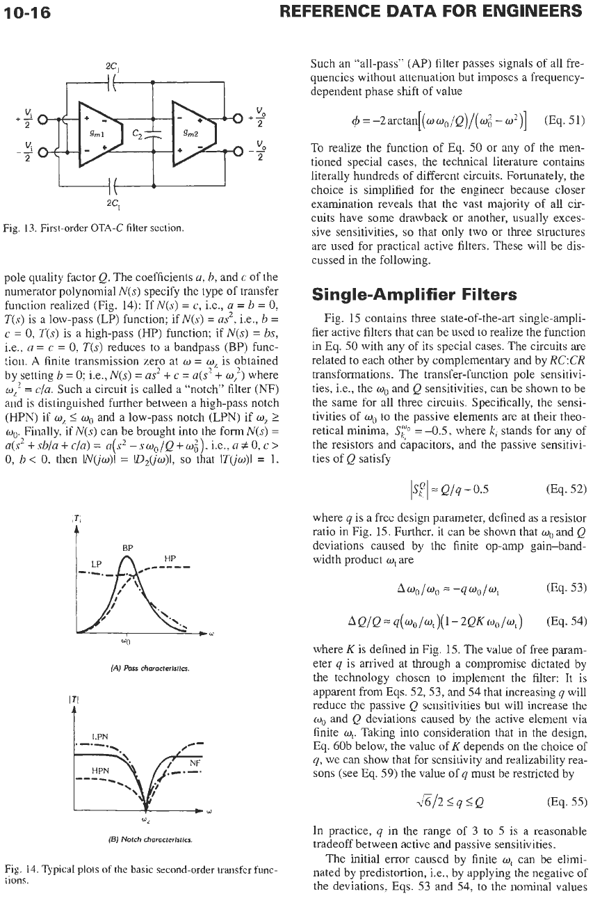
the form of
Eq.
19,
repeated here as
Eq.
48:
l/b
I
Fig.
12
shows different realizations of
a
function
of
l/(c-bJ
T(s)
=
V,
/V,
=
(as
+
b)/(s
+
e)
c
>
0
(Eq.
48)
Fig.
12A
is an appropriate realization if
0
I
a
I
1
and
0
5
b
5
e.
Note that in this case
T(s)
is realized by a pas-
sive
RC
network. The amplifier is
a
special case of Fig.
3B
for
Z,=
0
and Z,
=
m;
it is
a
buffer amplifier with
unity gain and very high input and zero output imped-
ance. The buffer has been included for the case in
which the
RC
network may have
a
significant load;
otherwise it can be omitted. Fig.
12B,
a
specialFase of
Fig.
3A,
realizes
-T(s);
the minus sign,
a
180
phase
shift, is immaterial in many applications. Fig.
12C
realizes
T(s)
for the case in which
a
2
1
and
0
I
c
I
b.
Finally, Fig.
12D
takes care of the case when
a
=
1
and
b
<
0,
i.e.,
~(s)
=
(s
-
lbl)/(s
+
e),
a
regime important
for all-pass functions (see below).
It
is
noted here that the circuits in Figs.
12B, 12C,
and
12D
realize Eq.
48
under the assumption of ideal
amplifiers.
As
discussed earlier, if the op amp is
described by
Eq.
8,
discrepancies from the ideal fre-
quency response must be expected. Fortunately, how-
ever, the majority of all cases require only the
realization of Eq.
48
with either
a
=
0
or
b
=
0.
Fig.
12A
can then always be used, possibly after factoring
out a multiplying (gain) constant that can be taken care
of in the remaining parts of the circuit. The unity-gain
buffer amplifier requires for perfect operation only
IA(jw)l>>
1,
as
can readily be seen from Eq.
11.
With
OTAs,
a
general and versatile first-order func-
tion can be implemented as shown in Fig.
13.
The fully
differential circuit realizes
K/V,
=
-(G
+g,,)/(sC,
+
gm2)
(Eq.
49)
Note that depending on the polarity of the transcon-
ductances and their connections, the values of
g,,
and
g,,
may be positive or negative
so
that zeros anywhere
in the s-plane and both inverting and noninverting
transfer functions can be realized.
SECOND-ORDER TRANSFER
FUNCTIONS
-THE
BIQUADS
Probably the most important basic building block
used in the design of active filters is the biquad,
a
sec-
ond-order circuit that realizes the transfer function of
Eq.
20,
which is repeated here
as
Eq.
50:
N(s)
-
as2
+
bs+c
D2(s)
(Eq.
50)
T(s)
=
~
-
s2
+
s
wo/Q
+
wi
-
(A)
For0
c
o
5
I
and
0
S
b
5
c.
(C)
For
(I
2
1
and
0
s
e
s
b.
(D)Fora=
landb<O.
Fig. 12.
Different realizations
of
T(s)
in
Eq.
48.
The
element
values
are
normalized resistors and capacitors.
where
wo
>
0
and
Q
>
0.
It
is standard practice
to
identify the coefficients of the second-order denomina-
tor polynomial
D2(s)
via the pole frequency
w,
and the
10-1
6
REFERENCE DATA FOR ENGINEERS
2CI
Fig. 13.
First-order OTA-C
filter
section.
pole quality factor Q. The coefficients
a,
b,
and
c
of the
numerator polynomial
N(s)
specify the type of transfer
function realized (Fig. 14): If
N(s)
=
c,
i.e.,
a
=
b
=
0,
~(s)
is a low-pass
(LP)
function; ifN(s)
=
as2,
i.e.,
b
=
c
=
0,
T(s)
is a high-pass
(HP)
function; if
N(s)
=
bs,
i.e.,
a
=
c
=
0,
T(s)
reduces
to
a bandpass
(BP)
func-
tion.
A
finite transmission zero at
w
=
w,
is obtained
by setting
b
=
0;
i.e.,
N(s)
=
as2
+
c
=
a(?
+
w:)
where
cor2
=
c/a. Such a circuit is called a “notch’ filter
(NF)
and
is
distinguished further between a high-pass notch
(HPN)
if
w,
5
wo
and a low-pass notch
(LPN)
if
w,
2
wo.
Finally, if
N(s)
can be brought into the form
N(s)
=
a(s2
+sb/a
+
c/u)
=
a(s2
-swo/e+w;),
i.e.,
azo,
c
>
0,
b
<
0,
then
IN(’jw)l
=
ID,(’jw)l,
so
that
ITuw)l
=
1.
li
BP
(A)
Pass
chamcterlstics.
w2
(E)
Notch chomcterfstics.
Fig.
14.
Typical plots
of
the
basic
second-order transfer func-
tions.
Such an “all-pass’’
(AP)
filter passes signals of all fre-
quencies without attenuation but imposes a frequency-
dependent phase shift of value
To realize the function of Eq. 50
or
any of the men-
tioned special cases,
the
technical literature contains
literally hundreds of different circuits. Fortunately, the
choice is simplified for the engineer because closer
examination reveals that the vast majority of all cir-
cuits have some drawback or another, usually exces-
sive sensitivities,
so
that only two or three structures
are used for practical active filters. These will be dis-
cussed in the following.
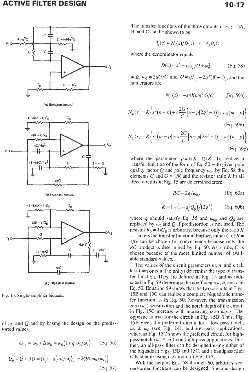
Single-Amplifier Filters
Fig. 15 contains three state-of-the-art single-ampli-
fier active filters that can be used to realize the function
in Eq. 50 with any of its special cases. The circuits are
related to each other by complementary and by
RCCR
transformations. The transfer-function pole sensitivi-
ties, Le., the
wo
and Q sensitivities, can be shown to be
the same for all three circuits. Specifically, the sensi-
tivities of
wo
to
the passive elements are at their theo-
retical minima,
Sp
=
-0.5, where
ki
stands for any of
the resistors and capacitors, and the passive sensitivi-
ties of Q satisfy
where
q
is a free design parameter, defined as a resistor
ratio in Fig. 15. Further, it can be shown that
wo
and
Q
deviations caused by the finite op-amp gain-band-
width product
w,
are
where
K
is defined in Fig. 15. The value of free param-
eter
q
is arrived at through a compromise dictated by
the technology chosen
to
implement the filter: It is
apparent from Eqs. 52,53, and 54 that increasing
q
will
reduce the passive Q sensitivities
but
will
increase the
wo
and Q deviations caused by the active element via
finite
w,.
Taking into consideration that in the design,
Eq. 60b below, the value of
K
depends on the choice of
q,
we can show that for sensitivity and realizability rea-
sons (see Eq.
59)
the value of
q
must be restricted by
In practice,
q
in the range
of
3
to
5
is a reasonable
tradeoff between active and passive sensitivities.
The initial error caused by finite
w,
can be elimi-
nated by predistortion, Le., by applying the negative of
the deviations, Eqs. 53 and 54, to the nominal values
10-1
7
The transfer functions of the three circuits
in
Fig. 15A,
B, and C can be shown to be
I;(s)
=
N,(s)/D(s)
i
=
A,
B,
C
where the denominator equals
D(s)=sZ+sw0/Q+o,'
0%.
58)
with
w,
=2qG/C and Q=q/[l-2q2(K-l)],andthe
numerators are
(A)
Bandpass biquod
(E)
Low-pas
blquad.
(l-k)(K- 1)Go GO
-
-
k(K-1)GO
nG
0
VZ
v10
4A-i
C (1-rn)C
11
I1
(l-n)G
-
-
rnC
If
I\
(CJ
Hlgh-pass blquad.
Fig.
15.
Single-amplifier
biquads.
of
o,
and
Q
and by basing the design
on
the predis-
torted values
w,,=wo+Aw,
=oo(l+qo0/wt) (Eq.56)
NA(s)
=
-s4Kmq2 G/C
(Eq. 59a)
(Eq. 59b)
(Eq. 59c)
where the parameter p=k(K-l)/K.
To
realize
a
transfer function of the form of
Eq.
50
with given pole
quality factor
Q
and pole frequency
w,,
by Eq. 58 the
elements
C
and G
=
1/R and the resistor ratio K in all
three circuits in Fig. 15 are determined from
RC
=
2q/woP (Eq. 60a)
K=1+(1-q/Qp)/(2q2)
0%.
6Ob)
where q should satisfy Eq.
55
and
mop
and
Qp
are
replaced
by
w,
and
Q
if predistortion is not used. The
resistor R,
=
1/G, is arbitrary, because
only
the ratio K
-
1 enters the transfer function. Further, either C or R
=
1/G can be chosen for convenience because
only
the
RC product is determined by Eq. 60. As a rule,
C
is
chosen because of the more limited number of avail-
able standard values.
The values of the circuit parameters m,
n,
and
k
(all
less than or equal to unity) determine the type of trans-
fer function. They are defined in Fig. 15 and
as
indi-
cated in
Eq.
59 determine the coefficients
a,
b,
and
c
in
Eq.
50.
Equation 59 shows that the two circuits in Figs.
15B and 15C can realize a complete biquadratic trans-
fer function
as
in
Eq.
50;
however, the transmission
zero
(a,)
sensitivities and the notch depth of the circuit
in Fig. 15C increase with increasing ratio
wz/wo.
The
opposite is true for the circuit in Fig. 15B. Thus, Fig.
15B gives the preferred circuit for
a
low-pass-notch,
w,
2
w,
(see Fig. 14), and low-pass applications,
whereas Fig. 15C shows the preferred circuit for high-
pass-notch
(0,
<
w,)
and high-pass applications. Fur-
ther, an all-pass filter can be designed using either of
the biquads in Figs. 15B and 15C, and a bandpass filter
is
best built using the circuit in Fig. 15A.
With the help of Eqs.
58
through 60, arbitrary sec-
ond-order functions can be designed. Specific design
10-1
8
REFERENCE DATA FOR ENGINEERS
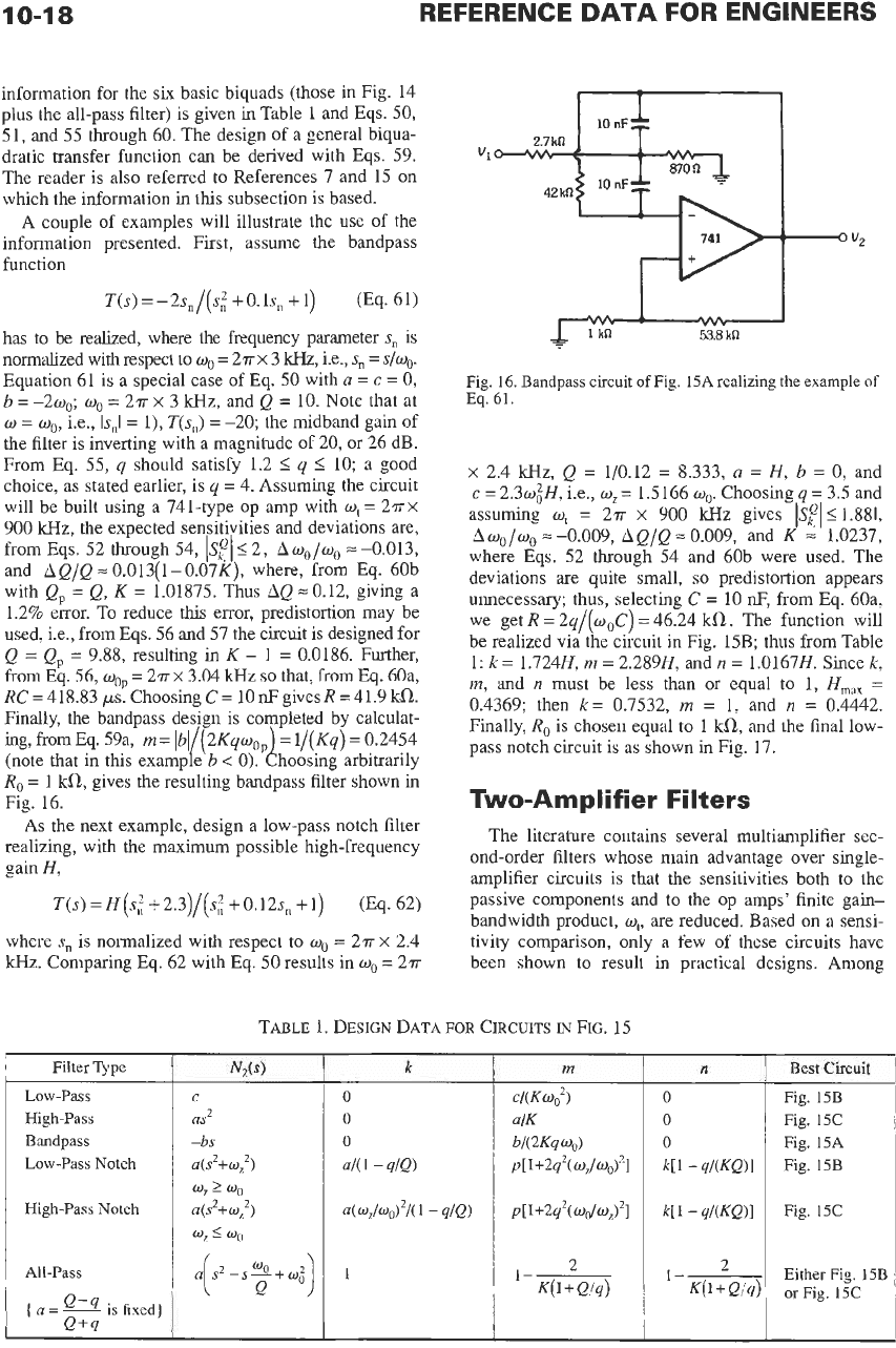
information for the six basic biquads (those in Fig. 14
plus the all-pass filter) is given in Table
1
and Eqs. 50,
5
1,
and 55 through 60. The design of a general biqua-
dratic transfer function can be derived with Eqs. 59.
The reader is also referred to References 7 and 15
on
which the information in this subsection
is
based.
A couple of examples will illustrate the use
of
the
information presented. First, assume the bandpass
function
T(s)=-2sn/(s2 +O.ls,
+1)
(Eq. 61)
has to be realized, where the frequency parameter
s,,
is
normalized with respect to
w,
=
25-x 3
kHz,
Le.,
s,,
=
s/wW
Equation 61 is
a
special case
of
Eq. 50 with
a
=
c
=
0,
b
=
-20,;
w,
=
25-
x
3
kHz,
and Q
=
10. Note that at
w
=
wo,
i.e.,
Is,I
=
l),
T(s,)
=
-20; the midband gain of
the filter is inverting with a magnitude
of
20, or 26 dB.
From Eq. 55,
q
should satisfy 1.2
4
q
4
10; a good
choice, as stated earlier, is
q
=
4. Assuming the circuit
will be built using
a
741-type op amp with
w,
=
25-
x
900
kHz,
the expected sensitivities and deviations are,
from Eqs. 52 through 54,
IS$<
2,
Awo/wo
=-0.013,
and AQ/Q =0.013(1-0.07K), where, from Eq. 60b
with Qp
=
Q, K
=
1.01875. Thus AQ
.-.
0.12, giving
a
1.2% error. To reduce
this
error, predistortion may be
used, i.e., from Eqs. 56 and 57 the circuit is designed for
Q
=
Qp
=
9.88, resulting in K
-
1
=
0.0186. Further,
from Eq. 56,
mop
=
27r
x
3.04
lCHz
so
that, from Eq. 60a,
RC=418.83 ps.ChoosingC= lOnFgivesR=41,9kCL.
Finally, the bandpass desi n is completed by calculat-
ing, from Eq. 59a,
m=
Ibl
2Kqw,,
=
l/(Kq)
=
0.2454
R,
=
1
kCL,
gives the resulting bandpass filter shown in
Fig. 16.
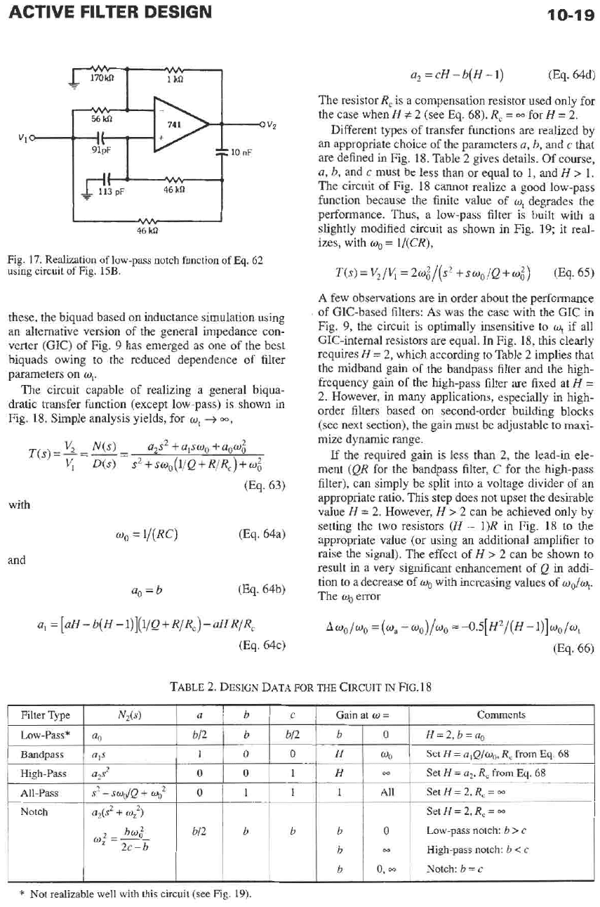
As the next example, design
a
low-pass notch filter
realizing, with the maximum possible high-frequency
gain H,
T(s)=H(s2+2.3)/(s2+0.12sn
+1) (Eq. 62)
where
s,
is normalized with respect to
w,
=
27r
x
2.4
kHz.
Comparing Eq. 62 with Eq. 50 results in
wo
=
27r
(note that in this examp
iB
e
b
<
0).
L
hoosing arbitrarily
53.8
kR
Fig.
16.
Bandpass circuit
of
Fig.
15A
realizing the example of
Eq.
61.
x
2.4
kHz,
Q
=
1/0.12
=
8.333,
a
=
H,
b
=
0,
and
c
=
2.3wiH, i.e.,
wz=
1.5166
wW
Choosing
q
=
3.5 and
assuming
w,
=
25-
x
900
kHz
gives
ISfl<l.SSI,
where Eqs. 52 through 54 and 60b were used. The
deviations are quite small,
so
predistortion appears
unnecessary; thus, selecting
C
=
10
I+,
from Eq. 60a,
we get
R
=
2q/(w0C)
=
46.24
kCL.
The function will
be realized via the circuit in Fig. 15B; thus from Table
1:
k
=
1.724H,
m
=
2.289H, and
n
=
1.0167H. Since
k,
m,
and
n
must be less than or equal to
1,
H,,,
=
0.4369; then
k=
0.7532,
m
=
1, and
n
=
0.4442.
Finally, R, is chosen equal to 1
kCL,
and the final low-
pass notch circuit is
as
shown in Fig. 17.
AwO/WO
=
-0.009, AQ/Q
=
0.009, and
K
=
1.0237,
Two-Amplifier
Filters
The literature contains several multiamplifier sec-
ond-order filters whose main advantage over single-
amplifier circuits is that the sensitivities both to the
passive components and to the op amps’ finite gain-
bandwidth product,
w,,
are reduced. Based on a sensi-
tivity comparison, only
a
few of these circuits have
been shown to result in practical designs.
Among
TABLE 1. DESIGN
DATA
FOR
CIRCUITS
IN
FIG.
15
1
Filter Type
1
N2(s)
I
k
I
rn
1
n
1
Bestcircuit
1
Low-Pass
High-Pass
Bandpass
Low-Pass
Notch
High-Pass Notch
Fig.
15B
Fig.
15C
1
Fig.
15A
Fig.
15B
I
I
Fig.
15C
1
Either Fig.
15B
’
orFig. 15C
j
ACTIVE FILTER DESIGN
Filter
Type
I
N2W
10-1
9
a
Iblcl
Gainatw=
1
Comments
a2
=cH-~(H-I)
(Eq. 64d)
The resistor
R,
is a compensation resistor used only for
the case when
H
f
2
(see Eq.
68). R,
=
w
for
H
=
2.
Different types of transfer functions
are
realized by
an appropriate choice of the parameters
a,
b,
and
c
that
are defined in Fig.
18.
Table
2
gives details. Of course,
a,
b,
and
c
must be less than or equal to
1,
and
H
>
1.
The circuit of Fig.
18
cannot realize a good low-pass
function because the finite value of
w,
degrades the
performance. Thus, a low-pass filter is built with a
slightly modified circuit as shown in Fig.
19;
it real-
izes, with
wo
=
l/(CR),
Bandpass
a,s
1
0
0
H
High-Pass
a,?
0 0
1
H
All-Pass
s'
-
swdQ
+
w:
0
1 1
1
"2
"1
I
Notch
...
46
kR
a2(s2
+
w,2)
Fig.
17.
Realization
of
low-pass notch function
of
Eq.
62
using circuit of
Fig.
15B.
wo
Do
All
0
m
0,
00
these, the biquad based
on
inductance simulation using
an alternative version of the general impedance con-
verter (GIC) of Fig.
9
has emerged as one of the best
biquads owing to the reduced dependence of filter
parameters
on
a,.
The circuit capable of realizing a general biqua-
dratic transfer function (except low-pass) is shown in
Fig.
18.
Simple analysis yields, for
wt
+
00,
Set
H
=
alQ/oo,
R,
from
Eq.
68
Set
H
=
a2, R,
from
Eq.
68
Set
H
=
2,
R,
=
M
SetH
=
2,
R,=
m
Low-pass notch:
b
>
c
High-pass notch:
b
<
c
Notch
b
=
c
wo
=
l/(RC)
(Eq. 64a)
and
a,=b
(Eq. 64b)
a,
=
[aH
-
b(H
-
l)](l/Q
+
R/R,)
-
aH
R/R,
(Eq. 64c)
A
few observations are in order about the performance
of GIC-based filters:
As
was the case with the GIC in
Fig.
9,
the circuit is optimally insensitive
to
wr
if all
GIC-internal resistors are equal. In Fig.
18,
this clearly
requires
H
=
2,
which according
to
Table
2
implies that
the midband gain of the bandpass filter and the high-
frequency gain of the high-pass filter are fixed at
H
=
2.
However, in many applications, especially in high-
order filters based
on
second-order building blocks
(see next section), the gain must be adjustable to maxi-
mize dynamic range.
If the required gain is less than
2,
the lead-in ele-
ment
(QR
for the bandpass filter,
C
for the high-pass
filter), can simply be split into a voltage divider of an
appropriate ratio. This step does not upset the desirable
value
H
=
2.
However,
H
>
2
can be achieved only by
setting the two resistors
(H
-
l)R
in Fig.
18
to the
appropriate value (or using an additional amplifier to
raise the signal). The effect
of
H
>
2
can be shown to
result in a very significant enhancement of
Q
in addi-
tion to a decrease of
wo
with increasing values of
wo/wt
The
wo
error
Awo/w0
=(ma
-wo)/wo
=-0.5[H2/(H-1)]wo/w,
(Eq.
66)
*
Not realizable
well
with this circuit
(see
Fig.
19).