Middleton W.M. (ed.) Reference Data for Engineers: Radio, Electronics, Computer and Communications
Подождите немного. Документ загружается.

10-20
REFERENCE
DATA
FOR ENGINEERS
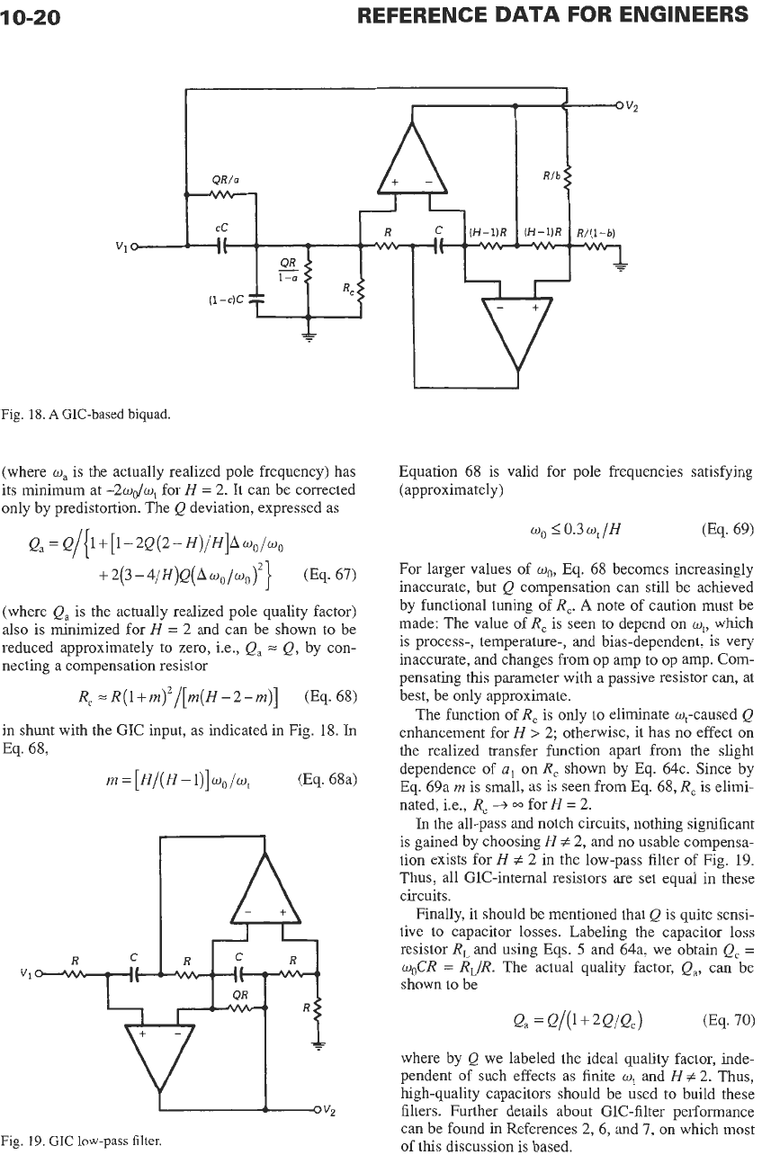
Fig.
18.
A
GIC-based biquad.
(where
wa
is the actually realized pole frequency) has
its minimum at
-2wdw,
for
H
=
2.
It can be corrected
only by predistortion. The
Q
deviation, expressed as
Q,
=
Q/[
1
+[I
-
2Q(2
-
H)/H]A
WO/~O
+2(3-4/H)Q(Awo/Uo)z}
(Eq.
67)
(where
Q,
is the actually realized pole quality factor)
also is minimized for
H
=
2
and can be shown to be
reduced approximately to zero, i.e.,
Q,
=
Q,
by con-
necting
a
compensation resistor
R,
=
R(1+m)2/[rn(H-2-m)]
(Eq. 68)
in shunt with the GIC inuut, as indicated in Fig.
18.
In
n
(Eq. 68a)
-
v2
Fig.
19.
GIC low-pass filter.
Equation 68 is valid for pole frequencies satisfying
(approximately)
For larger values of
wo,
Eq. 68 becomes increasingly
inaccurate, but
Q
compensation can still be achieved
by functional tuning of
R,.
A
note of caution must be
made: The value of
R,
is seen to depend
on
w,,
which
is process-, temperature-, and bias-dependent,
is
very
inaccurate, and changes from op amp to op amp. Com-
pensating
this
parameter with a passive resistor can, at
best, be only approximate.
The function of
R,
is only to eliminate wt-caused
Q
enhancement for
H
>
2;
otherwise, it has
no
effect
on
the realized transfer function apart from the slight
dependence of
al
on
R,
shown by Eq. 64c. Since by
Eq. 69a
m
is small, as is seen from Eq. 68,
R,
is elimi-
nated, i.e.,
R,
+
w
for
H
=
2.
In
the all-pass and notch circuits, nothing significant
is gained by choosing
H
#
2,
and
no
usable compensa-
tion exists for
H
f
2
in the low-pass filter
of
Fig.
19.
Thus, all GIC-internal resistors are set equal in these
circuits.
Finally, it should be mentioned that
Q
is
quite sensi-
tive to capacitor losses. Labeling the capacitor
loss
resistor
R,
and using Eqs.
5
and 64a, we obtain
Q,
=
woCR
=
RJR.
The actual quality factor,
Qa,
can be
shown to be
where by
Q
we labeled the ideal quality factor, inde-
pendent
of
such effects as finite
wr
and
H
#
2.
Thus,
high-quality capacitors should be used to build these
filters. Further details about GIC-filter performance
can be found in References
2,
6, and
7,
on
which most
of this discussion is based.
ACTIVE
FILTER
DESIGN
1
0-2
1
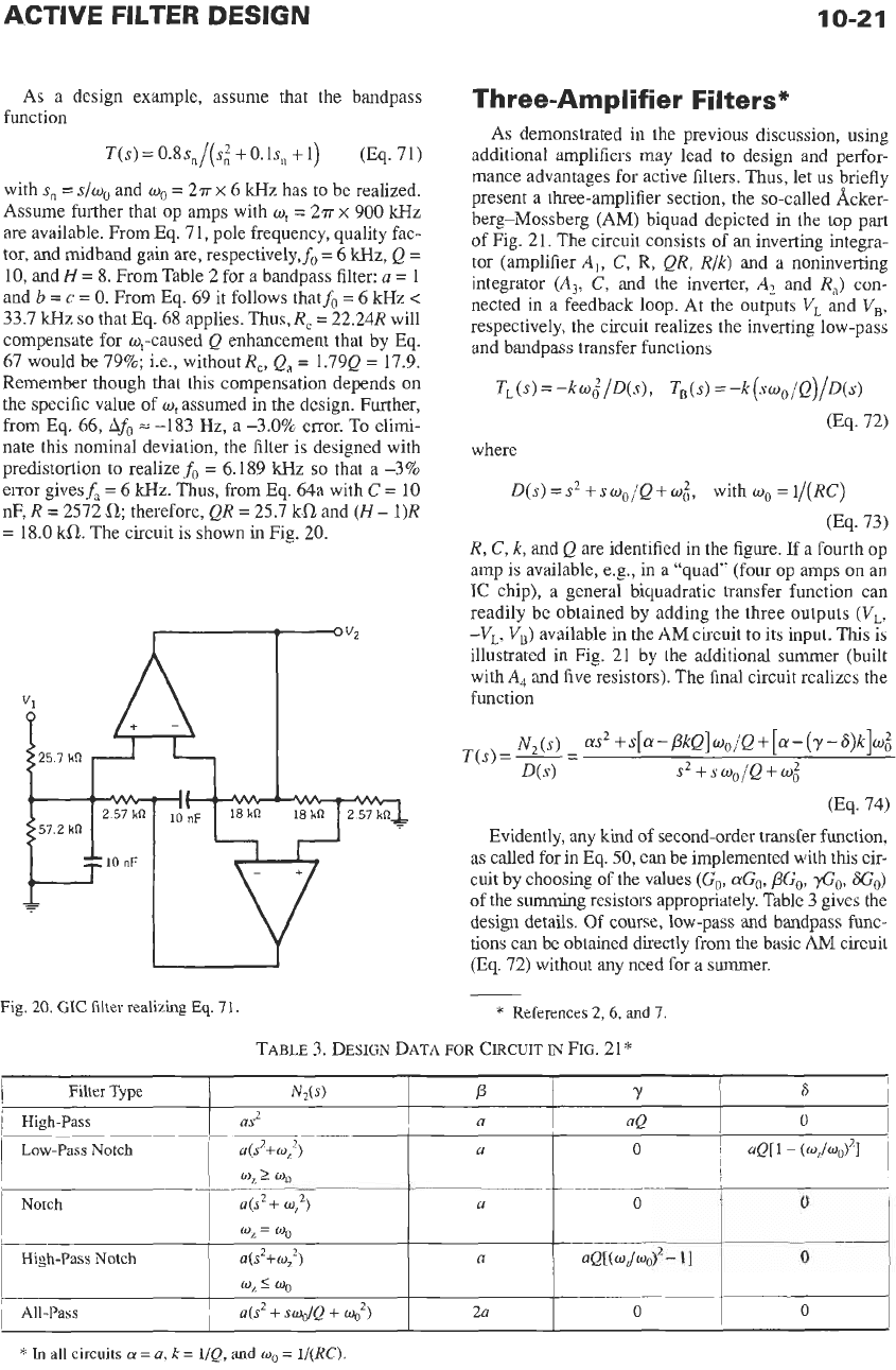
As a design example, assume that the bandpass
T(s)=0.8sn/(s~+O.ls,
+1)
(Eq.
71)
with
s,
=
s/wo
and
wn
=
2a
x
6
kHz
has to be realized.
Assume further that op amps with
w,
=
27r
x
900
Wz
are
available. From Eq.
7
1,
pole frequency, quality fac-
tor, and midband gain are, respectively,fn
=
6
kHz,
Q
=
10,
and
H
=
8.
From Table
2
for a bandpass filter:
a
=
1
and
b
=
c
=
0.
From Eq.
69
it follows thatf,
=
6 kHz
<
33.7
Wz
so that Eq.
68
applies. Thus,
R,
=
22.2413
will
compensate for w,-caused
Q
enhancement that by Eq.
67
would be
79%;
Le., without
R,, Q,
=
1.79Q
=
17.9.
Remember though that this compensation depends on
the specific value of
w,
assumed in the design. Further,
from Eq.
66,
AfO
=
-183
Hz,
a
-3.0%
error. To elimi-
nate this nominal deviation, the filter is designed with
predistortion to realizef,
=
6.189
kHz
so
that a
-3%
error givesf,
=
6
kHz. Thus, from Eq.
64a
with
C
=
10
nF,
R
=
2572
0,
therefore,
QR
=
25.7
kCl
and
(H
-
l)R
=
18.0
kCl.
The circuit is shown in Fig.
20.
function
Fig.
20.
GIC
filter realizing
Eq.
71.
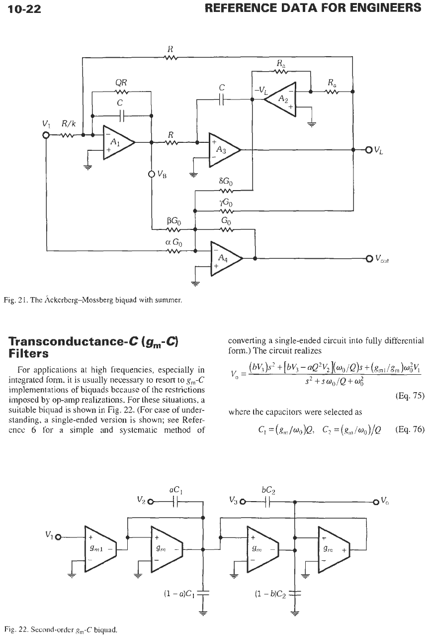
Three-Amplifier Filters*
As demonstrated in the previous discussion, using
additional amplifiers may lead
to
design and perfor-
mance advantages €or active filters. Thus, let
us
briefly
present a three-amplifier section, the so-called Acker-
berg-Mossberg (AM) biquad depicted in the top part
of Fig.
21.
The circuit consists of an inverting integra-
tor (amplifier
A,,
C,
R,
QR,
R/k)
and a noninverting
integrator
(A3,
C,
and the inverter,
A,
and
R,)
con-
nected in a feedback loop. At the outputs
VL
and
V,,
respectively, the circuit realizes the inverting low-pass
and bandpass transfer functions
where
D(s)=s2+swO/Q+w;,
with
wn
=l/(RC)
R,
C,
k,
and
Q
are identified in the figure. If a fourth
op
amp
is available, e.g., in a “quad” (four op amps
on
an
IC
chip), a general biquadratic transfer function can
readily be obtained by adding the three outputs
(VL,
-VL, V,)
available in the AM circuit to its input. This is
illustrated in Fig.
21
by the additional summer (built
with
A,
and five resistors). The final circuit realizes the
function
(Eq.
73)
N
(s)
D(s)
as2
+
$[a
-
PkQ]
wo/Q
+
[a
-
(7-
S)k]w;
(Eq.
74)
T(s)
=
2
=
s2
+
swo/Q
+
wo’
Evidently, any kind
of
second-order transfer function.
as called for in Eq.
50,
can be implemented with
this
cir-
cuit by choosing of the values
(GO,
aG,,
PGn,
fin,
SC,)
of the summing resistors appropriately. Table
3
gives the
design details. Of couse, low-pass and bandpass func-
tions can be obtained directly
fi-om
the basic
AM
circuit
(Eq.
72)
without any need for a summer.
*
References
2,6,
and
7.
TABLE
3.
DESIGN DATA
FOR
CIRCUIT
W
FIG.
2 1
‘’
*
In
all
circuits
(Y
=
a,
k
=
l/Q,
and
wo
=
l/(RC).
10-22
REFERENCE
DATA
FOR ENGINEERS
GO
vvv
I
Fig.
21.
The
&kerberg-Mossberg biquad
with
summer.
converting
a
single-ended circuit
into
fully differential
form.) The circuit realizes
Trans
co
n
d
u
c
t
a
n
ce-
C
(
g,-
C)
Filters
For
applications
at
high frequencies, especially in
integrated
form,
it
is
usually necessary to resort to
g,-C
implementations of biquads because of the restrictions
imposed by op-amp realizations.
For
these situations, a
suitable biquad is shown in Fig.
22. (For
ease
of
under-
standing, a single-ended version is shown; see Refer-
ence
6
for a simple and systematic method of
",
=
(bV3)s2
+[b%
-aQ'v,](o,/Q)s+(g,i/g,)w~V,
s2+soo/Q+o,'
0%.
75)
where the capacitors were selected
as
Ci
=(g,/oo)Q,
G
=(gm/~o)/Q
(Eq.76)
Fig.
22.
Second-order
gm-C
biquad.
ACTIVE FILTER DESIGN
10-23
and, therefore,
oo
=
gm/G
and
Q
=
a
(Eq.
77)
Depending on whether the input
V,,
is applied to the
terminal
V,,
V,,
and/or
V3,
the circuit in Fig. 22 can
realize any type of second-order function.
In
particu-
lar, a fully biquadratic function can be obtained by set-
ting
V,
=
V,
=
V,
=
vn.
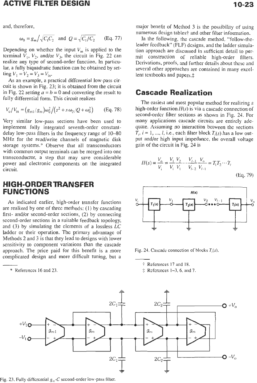
As an example, a practical differential low-pass cir-
cuit is shown in Fig. 23; it is obtained from the circuit
in Fig.
22
setting
a
=
b
=
0
and converting the result to
fully differential form. This circuit realizes
Very similar low-pass sections have been used to
implement fully integrated seventh-order constant-
delay low-pass filters in the frequency range of 10-80
MHz for the read/write channels
of
magnetic disk
storage systems.
*
Observe that all transconductors
with common output terminals can be merged into one
transconductor, a step that may save considerable
power and electronic components on the integrated
circuit.
HIGH-ORDER TRANSFER
FUNCTIONS
As indicated earlier, high-order transfer functions
are realized by one
of
three methods: (1) by cascading
first- and/or second-order sections,
(2)
by connecting
second-order sections in a suitable feedback topology,
and (3) by simulating the elements of a lossless
LC
ladder or their operation. The primary advantage of
Methods 2 and 3 is that they lead to designs with lower
sensitivity to component variations than the cascade
approach. The price paid for this benefit is a more
complicated design and more difficult tuning, but a
*
References
16
and
23.
major benefit of Method 3 is the possibility of using
numerous design tables? and other filter information.
In
the following, the cascade method, “follow-the-
leader feedback” (FLF) designs, and the ladder simula-
tion approach are discussed in sufficient detail to per-
mit construction of reliable high-order filters.
Derivations, proofs, and further details about these and
several other approaches are contained in many excel-
lent textbooks and papers.$
Cascade Realization
The easiest and most popular method for realizing a
high-order function
H(s)
is via a cascade connection of
second-order filter sections as shown in Fig. 24. For
many applications cascade circuits are entirely ade-
quate. Assuming no interaction between the sections
TL,
i
=
1,
...,
1,
Le., each filter block
T,(s)
has a low out-
put and/or high input impedance, the overall voltage
gain of the circuit in Fig.
24
is
Fig.
24.
Cascade connection of blocks
T,(s).
f
References
17
and
18.
$
References
1-3,
6,
and
7
-
1
0
-vo
Fig.
23.
Fully
differential
g,-C
second-order low-pass filter.
10-24
REFERENCE
DATA
FOR ENGINEERS
To
this end, Eq. 17 is factored into the product of
I
sec-
ond-order transfer functions
T,(s)
=
N,(s)/D,(s)
of the
form of Eq. 50, such that
1 1
N(s)
=
nNi(s),
D(s)
=
nDi(s)
(Eq.
80)
i=l
i=l
This step is accomplished simply by finding the (in
general) complex roots of
N(s)
and
D(s)
and keeping
conjugate complex terms together
so
that all coeffi-
cients in
T,(s)
are real.
The notation in Eqs. 17, 79, and
80
has tacitly
assumed that
H(s)
is of even order, Le., that
r
is even.
Of course, if
r
is odd, one of the transfer functions
T,(s)
in Eq. 79 must be of first order; that is, it must be of the
form of Eq.
48,
whose realizations are given in Figs.
12 and
13.
Such a first-order function can always be
cascaded with the remainder of the network. If in Eq.
17
m
<
r,
some of the terms
N,(s)
in Eq.
80
are fre-
quency independent constants
so
that the correspond-
ing biquads are low-pass functions. Thus, it should be
clear that the discussion can concentrate on the synthe-
sis of even-order functions only; i.e., the question is
how to realize Eq. 17 as expressed in Eq. 79 with Eq.
80.
This, in
turn,
implies that practical methods have to
be found to realize biquadratic transfer functions of the
form of Eq. 50, a topic discussed
in
the previous sec-
tion
of
this chapter.
As
a
simple example for the steps discussed, assume
the function
K(s’
+
4rr’
x
3.3551)
s4
+
2.7555~~
+
3.7964s’
+
3.099s
+
1.4246
H(s)
=
(Eq.
81)
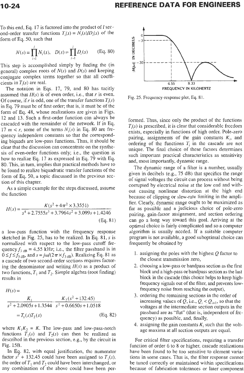
a low-pass function with the frequency response
sketched in Fig. 25, has to be realized. In Eq. 81,
s
is
normalized with respect to the low-pass cutoff fre-
quencyf3
dB
=
4.55 kHz; Le., the filter passband is in
0
5f5f3dB,
and
s
=
j0/(2rx
f3
*).
Realizing Eq.
81
as
a cascade of two second-order sections requires factor-
ing the denominator and writing
H(s)
as a product of
two functions,
TI
and
T2.
Simple algebra (root finding)
results in
H(s)
=
K,
K,(s2
+132.45)
s2
+2.0905s+1.3544
s2
+0.6650s+1.0518
where
K1K2
=
K.
The low-pass and low-pass-notch
functions
T,(s)
and
T,(s)
can then be realized as
described in the previous section, e.g., by the circuit in
Fig. 15B.
In
E 82, with equal justification, the numerator
factors
+
132.45 could have been assigned
to
T,(s),
the order of
TI
and
T,
could have been interchanged, or
any combination of the above could have been per-
4.
FREQUENCY
IN
KILOHERTZ
Fig.
25.
Frequency-response plot,
Eq.
81.
formed. Thus, since only the product of the functions
T,(s)
is prescribed, it is clear that considerable freedom
exists, especially in functions of high order. Pole-zero
pairing, assignments of the gain constants
K,,
and
ordering of the functions
T,
in
the cascade are not
unique. The final choice of these factors determines
such important practical characteristics as sensitivity
and, most importantly, dynamic range.
The dynamic range of a filter is a number, usually
given in decibels (e.g., 75 dB) that specifies the range
of signal voltages the circuit can process without being
corrupted by electrical noise at the low end and with-
out causing nonlinear distortion at the high end
because of clipping or slew-rate limiting in the ampli-
fier. Clearly, dynamic range ought to be maximized as
far as possible and a judicious choice of pole-zero
pairing, gain-factor assignment, and section ordering
can go a long way toward this goal. Arriving at the
optimal choice is fairly complicated and
so
a computer
algorithm is usually needed.
If
a suitable computer
program is not available, a good suboptimal choice can
frequently be obtained by
1.
assigning the poles with the highest
Q
factor to
the closest transmission zero,
2. choosing a low-pass or bandpass section as the first
block and a high-pass or bandpass section as the last
block in the cascade
(this
choice helps to keep high-
frequency signals out
of
the filter, and prevents low-
frequency noise
from
reaching
the
output),
increasing values of
Q,
i.e.,
Q,
<
Qi+l,
so
that the
voltages at the intermediate section outputs in the
passband are as “flat” (that is, independent of fre-
quency) as possible, and, finally,
4. assigning the gain constants
K,
such that the volt-
age maxima at all section outputs are equal.
For critical filter specifications, requiring a transfer
function of order 6 to
8
or higher, cascade realizations
have been found to be too sensitive to element varia-
tions in some cases. That
is,
the filter response cannot
be tuned correctly or maintained within specifications
because of fabrication tolerances or later component
3.
ordering the remaining sections in the order of
ACTIVE
FILTER
DESIGN
10-25
changes, such as those caused by aging or temperature
drifts. Such sensitivity problems are particularly severe
in
filters with high-Q (narrow bandwidth or steep roll-
off
from passband
to
stopbands). For these cases, fre-
quently, multiple-feedback topologies give useful
solutions. For very critical and stringent filter specifi-
cations, active simulations of passive
LC
ladder filters
show the best sensitivity performance and are pre-
ferred as alternative realizations.
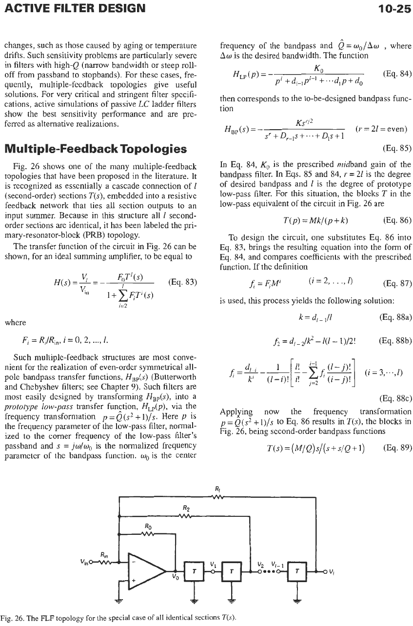
Multiple-Feedback Topologies
Fig. 26 shows one of the many multiple-feedback
topologies that have been proposed in the literature. It
is recognized as essentially a cascade connection of
1
(second-order) sections
T(s),
embedded into a resistive
feedback network that ties all section outputs
to
an
input summer. Because in this structure all
1
second-
order sections are identical, it has been labeled the pri-
mary-resonator-block
(PRB)
topology.
The transfer function of the circuit in Fig. 26 can be
shown, for an ideal summing amplifier,
to
be equal
to
H(s)
2
-
FoT'(s)
I
(Eq.
83)
l+CqT'(s)
i=2
where
Fi
=
Ri/Rin,
i
=
0,
2,
...,
1.
Such multiple-feedback structures are
most
conve-
nient for the realization of even-order symmetrical all-
pole bandpass transfer functions,
HBp(s)
(Butterworth
and Chebyshev filters; see Chapter
9).
Such filters are
most easily designed by transforming
HBp(s),
into a
prototype low-pass
transfer function,
HLp(p),
via the
frequency transformation
p
=
Q(s2
+
I)/s. Here
p
is
the frequency parameter of the low-pass filter, normal-
ized
to
the comer frequency of the low-pass filter's
passband and
s
=
jw/wO
is the normalized frequency
parameter of the bandpass function.
wO
is the center
frequency of the bandpass and
Q
=
wO/Aw
,
where
A@
is the desired bandwidth. The function
0%.
84)
KO
HLP (PI
=
-
p'+d,-,p'-'
+...
dlp+dO
then corresponds to the to-be-designed bandpass func-
tion
Ks'I2
HBP(S)
=
-
(r
=
21
=
even)
s'
+
D,-,S
+
...
+
Dp
+
1
0%.
85)
In
Eq.
84,
KO
is the prescribed midband gain of the
bandpass filter.
In
Eqs.
85
and
84,
r
=
21
is the degree
of desired bandpass and
1
is the degree of prototype
low-pass filter.
For
this situation, the blocks
T
in the
low-pass equivalent of the circuit in Fig. 26 are
T(P)
=
Mk/(P
+
k)
0%.
86)
To
design the circuit, one substitutes Eq. 86 into
Eq.
83,
brings the resulting equation into the form of
Eq.
84,
and compares coefficients with the prescribed
function. If the definition
(Eq.
87)
=<Mi
(i
=
2,
.
.
./
I)
is used, this process yields the following solution:
k=d/-,ll
(Eq. 88a)
f2
=
d,-&
-
l(1-
1)/2!
(Eq. 88b)
(Eq. 8%)
Applying now the frequency transformation
p
=
Q
(s2
+
l)/s
to
Eq. 86 results in
T(s),
the blocks in
Fig.
26,
being second-order bandpass functions
T(s)
=(M/Q)s/(s+siQ+l)
0%.
89)
RI
I
R2
I
Fig.
26.
The FLF topology
for
the special case
of
all
identical sections
T(s).
1
Q-26
REFERENCE
DATA
FOR ENGINEERS
where
Q
=
Ql/d,-I
is the quality factor of
T(s),
Le.,
wo
divided by the
3-dB
bandwidth of
T.
Note that all
blocks
T(s)
are tuned to the same
oo
because
s
=
jo/wo.
The gain constant
M
of
T(s)
should be selected for best
dynamic range, such that all filter-internal signal max-
ima are equal.
In
general,
this
requires a computer rou-
tine and results in different
M
factors for each section;
a good suboptimal choice, however, which at the same
time retains
all
identical sections,
is
simply
M
=
41
+
[Q/Qr
(Eq. 90)
With
M
and&,
i
=
2,
...,
I,
known from Eqs.
88
and 90,
the actual feedback factors
F,
=
R,/R,,
can then be
determined from Eq. 87. Finally, the
PRB
bandpass
design is completed by setting
F,
=
R,/R,,
=
(Ko/M')(Q/Q)'
(Eq. 91)
so
that the prescribed gain constant
KO
is realized cor-
rectly.
An
example will illustrate the process:
To
be
designed is a sixth-order bandpass filter with a Butter-
worth magnitude characteristic, center frequency
fo
=
4.8 kHz, center-frequency gain
KO
=
5 (14
dB),
and
3-dB
bandwidth
Af
=
600 Hz. For this case, the prototype
third-order Butterworth low-pass transfer function,
corresponding
to
Eq. 84, is
HLp(p)=-5/(p3
+2p2+2p+1) (Eq. 92)
apd the low-pass-to-bandpass transformation, with
Q
=
4.8
kHz/0.6
kHz
=
8,
is
p
=
8(s2
+
l)/s
(Eq. 93)
where
s
=
j
w/(2~
x
4.8 kHz). Then, from Eqs. 87 and
92,
k
=
2/3,
fi
=
1.5,
and
f,
=
0.875. From Eqs. 89 and
90, the second-order sections have a pole quality factor
Q
=
8
x
3/2
=
12
and a gain constant
M
=
[
1
+
(3/2)2]"2
=
1.8028; that is, the functions to be realized are
T(s)=0.1502s/(s2 +s/12+1) (Eq. 94)
Finally, the feedback resistor ratios
F,
are, from Eq. 87,
F2
=
f2/M
=
0.46 15 and
F,
=
f3/M
=
0.1493 and from
Eq. 91,
Fo
=
2.880.
The single-amplifier bandpass filter of Fig.
15A
will
be used to realize the function of Eq. 94. The design is
completed as follows: From Eqs. 59, 56, and 57 with a
choice of
q
=
5,
one obtains
K
=
1.01149 and the pre-
distorted values, iff,
=
1
MHz,
fnp
=
4.915 Hz, and
Q,
=
11.75. If
C
=
12
nF
is chosen, Eq. 58 yields
R
=
27.0
kQ. Finally, from Table
1,
with
Ibl
=
0.15020,,,
m
=
0.0149
=
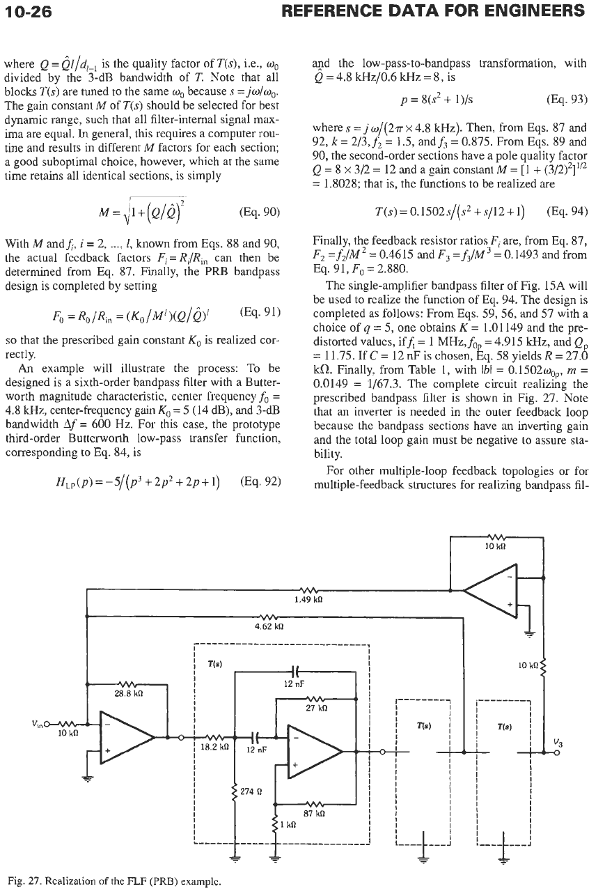
1/67.3. The complete circuit realizmg the
prescribed bandpass filter is shown
in
Fig. 27. Note
that
an
inverter is needed in the outer feedback loop
because the bandpass sections have an inverting gain
and the total loop gain must be negative to assure sta-
bility.
For other multiple-loop feedback topologies or for
multiple-feedback structures for realizing bandpass fil-
Fig.
10-27
ters with finite transmission zeros, the reader is referred
to the literature.*
Ladder Simulation
Doubly terminated passive
LC
ladder filters are
known to be optimally insensitive to element varia-
tions. Thus, in recent years, many methods have been
proposed that simulate the operation, the topology,
and/or the elements of
LC
ladders by active networks.
The goal is to eliminate inductors and, at the same
time,
to
retain the ladder's superior sensitivity perfor-
mance. A few simple but powerful procedures are
described in the following; for more details and for the
design
of
very demanding filter circuits, the reader is
referred to the 1iterature.t
Operational Simulation-The process of simulat-
ing the operation of an
LC
ladder is best explained by
an example from which the general design procedure
should become clear.
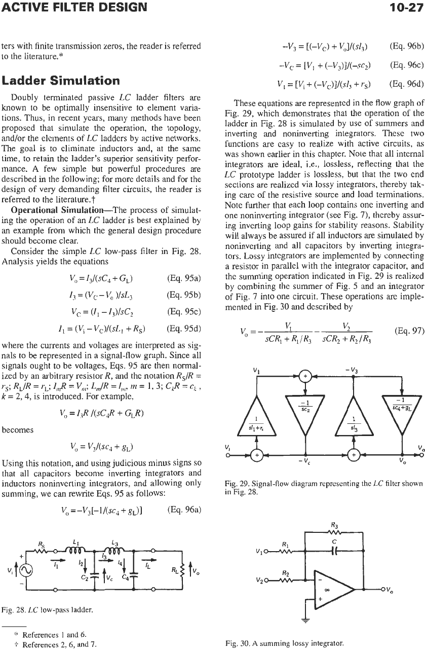
Consider the simple
LC
low-pass filter in Fig. 28.
Analysis yields the equations
(Eq. 95a)
(Eq. 95b)
(Eq. 95c)
V,
=
13/(sCq
+
GJ
13
=
(VC
-
v,
)/sL3
vc
=
(11
-
13)/SC2
1,
=
(V,
-
V~)/(SL,
+
R,)
(Eq. 95d)
where the currents and voltages are interpreted as sig-
nals to be represented in a signal-flow graph. Since all
signals ought to be voltages, Eqs. 95
are
then normal-
ized by an arbitrary resistor
R,
and the notation
R,IR
=
us;
RJR
=
u,;
Z,$
=
V,;
L,/R
=
l,,
m
=
1,
3;
C$
=
ck
,
k
=
2,4,
is introduced. For example,
V,
=
13R /(sC,R
+
G,R)
becomes
v,
=
V3/(%
+
gd
Using this notation, and using judicious minus signs
so
that all capacitors become inverting integrators and
inductors noninverting integrators, and allowing only
summing, we can rewrite Eqs. 95 as follows:
V, =-V3[-l/(sc, +gL)]
(Eq. 96a)
-Vc
=
[Vi
+
(-VJ]/(-SCZ)
(Eq. 96~)
VI
=
[Vi
+
(-Vc)]/(~l3
+
Y,)
(Eq. 96d)
These equations are represented in the flow graph of
Fig. 29, which demonstrates that the operation of the
ladder in Fig. 28 is simulated by use
of
summers and
inverting and noninverting integrators. These two
functions are easy to realize with active circuits, as
was shown earlier in
this
chapter. Note that all internal
integrators are ideal, Le., lossless, reflecting that the
LC
prototype ladder is lossless, but that the two end
sections are realized via lossy integrators, thereby tak-
ing care of the resistive source and load terminations.
Note further that each loop contains one inverting and
one noninverting integrator (see Fig. 7), thereby assur-
ing inverting loop gains for stability reasons. Stability
will always be assured if all inductors
are
simulated by
noninverting and all capacitors by inverting integra-
tors. Lossy integrators are implemented by connecting
a resistor in parallel with the integrator capacitor, and
the summing operation indicated in Fig. 29 is realized
by combining the summer of Fig.
5
and an integrator
of Fig.
7
into one circuit. These operations are imple-
mented in Fig.
30
and described by
(Eq. 97)
v,=-
-
v2
sCR,
+
R,
/
R3 sCR,
+
R2
f
R3
V1
-
"3
I
I
Fig.
29.
Signal-flow diagram representing the
LC
filter shown
in Fig.
28.
Fig.
28. LC
low-pass ladder.
*
References
1
and
6.
t
References
2,6,
and
I.
Fig.
30.
A
summing
lossy
integrator.
10-28
REFERENCE
DATA
FOR ENGINEERS
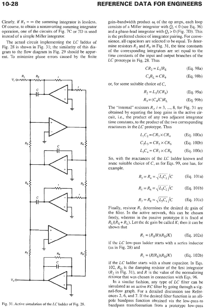
Clearly, if
R3
=
M
the summing integrator is lossless.
Of
course, to obtain a noninverting summing integrator
operation, one of the circuits of Fig. 7C or
7D
is used
instead of a simple Miller integrator.
The actual circuit implementing the
LC
ladder
of
Fig. 28
is
shown in Fig.
31;
the similarity of this dia-
gram to the flow diagram in Fig. 29 should be appar-
ent.
To minimize phase errors caused by the finite
+
C
R‘
Fig.
31.
Active simulation
of
the
LC
ladder
of
Fig.
28.
gain-bandwidth product
q
of the op amps, each loop
consists of a Miller integrator with
QI
<
0
(see Eq.
36)
and a phase-lead integrator with
Q,>
0
(Fig.
7D).
This
is the preferred choice of integrator pairing. For conve-
nience, all capacitors are selected to be equal.
To
deter-
mine resistors
R2
and
R,
in Fig.
31,
the time constants
of the corresponding integrators are set equal to the
time constants of the input and output branches of the
LC
prototype in Fig. 28. Thus
CR2
=
Ll/Rs
(Eq. 98a)
C4RL
=
CR,
(Eq. 98b)
or, for some suitable choice
of
C,
R2
=
Ll/(CRs)
(Eq. 99a)
R,
=
(CdCIRL
(Eq. 99b)
The “internal” resistors
Ri,
i
=
3,
...,
8,
for Fig.
31
are
obtained by equating the loop gains in the active cir-
cuit, i.e., the product of any two adjacent integrator
time constants, to the product of the two corresponding
reactances
in
the
LC
prototype. Thus
LIC2
=
CR3
x
CR,
(Eq. 100a)
C2L3
=
CR,
X
CR,
(Eq. 100b)
L3C4
=
CR7
x
CR,
(Eq. 1OOc)
So,
with the reactances of the
LC
ladder known and
some suitable choice of
C,
as for Eqs. 99, one has, for
example,
R3
=
R,
=
m/C
(Eq. 101a)
R5
=
R,
=
G/C
(Eq. 101b)
R7
=
R8
=
G/C
(Eq. 101~)
Finally, resistor
Rl
determines the desired dc gain of
the filter.
In
the active network, this can be chosen
freely, whereas in the passive prototype it is fixed at
RJ(R,
+
RL).
Let the dc gain be called
K,
then it can be
shown that
Rl
=
(RS/R)(R,/K)
(Eq. 102a)
if the
LC
low-pass ladder starts with
a
series inductor
(as in Fig.
28)
and
Rl
=
(R/RS)(RD/K)
(Eq. 102b)
if the
LC
ladder starts with a shunt capacitor.
In
Eqs.
102,
RD
is the damping resistor of the first integrator
(R2
in Fig.
31),
and
R
is the value of the normalizing
resistor that was chosen in connection with Eqs. 96.
In a similar fashion, any type of
LC
filter can be
simulated as an active
RC
filter by going through a sig-
nal-flow graph. For a detailed discussion see Refer-
ences 2,6, and 7.
If
the desired filter function
is
an all-
pole bandpass function obtained via the low-pass-to
bandpass transformation from a prototype low-pass
ACTIVE
FILTER
DESIGN
10-29
function,
as
illustrated in connection with the transfor-
mation from Eq.
84
to Eq.
85,
the design is particularly
simple. One only needs to simulate the low-pass filter
by a signal-flow graph,
as
shown in Fig. 29 for a
fourth-order case, and then use the low-pass-to-band-
pass transformation to transform each integrator of the
form
Ti@)
=
a/(@
+
c)
into a second-order bandpass
section
T(s)
=
[~~/(bQ)]/[s+sc/(bQ)+l]
(Eq.
103)
similar to the transformation from Eq.
86
to Eq.
89
above. For ideal integrators, the coefficient
c
=
0,
implying a bandpass of infinite
Q*
for all internal sec-
tions of the simulated ladder (compare Fig. 29). After
a
suitable realization for the second-order sections is
obtained
as
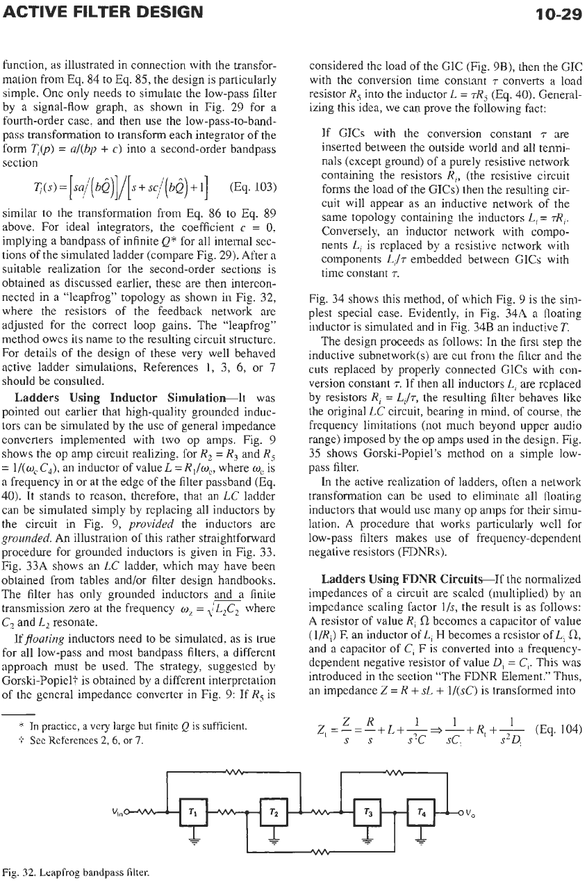
discussed earlier, these are then intercon-
nected in a “leapfrog” topology
as
shown in Fig.
32,
where the resistors of the feedback network are
adjusted for the correct loop gains. The “leapfrog”
method owes its name to the resulting circuit structure.
For details of the design of these very well behaved
active ladder simulations, References
1,
3, 6,
or
7
should be consulted.
Ladders Using Inductor Simulation-It was
pointed out earlier that high-quality grounded induc-
tors can be simulated by the use of general impedance
converters implemented with two op amps. Fig.
9
shows the op amp circuit realizing, for
R,
=
R,
and
R,
=
l/(q
CJ,
an inductor of value
L
=
R,/w,,
where
w,
is
a
frequency in or at the edge of the filter passband (Eq.
40).
It stands
to
reason, therefore, that an
LC
ladder
can be simulated simply by replacing all inductors by
the circuit in Fig.
9,
provided the inductors are
grounded.
An
illustration of this rather straightforward
procedure for grounded inductors is given in Fig.
33.
Fig.
33A
shows
an
LC
ladder, which may have been
obtained from tables and/or filter design handbooks.
The filter has only grounded inductors and a finite
transmission zero at the frequency
w,
=
+&
where
C,
and
L,
resonate.
Iffloating inductors need to be simulated,
as
is true
for all low-pass and most bandpass filters,
a
different
approach must be used. The strategy, suggested by
Gorski-Popiel-f is obtained by a different interpretation
of the general impedance converter in Fig.
9:
If
R,
is
I
*
In practice,
a
very
large
but
finite
Q
is
sufficient.
i-
See
References
2,
6,
or
7.
considered the load of the GIC (Fig.
9B),
then the GIC
with the conversion time constant
T
converts a load
resistor
R,
into the inductor
L
=
TR,
(Eq.
40).
General-
izing this idea, we can prove the following fact:
If GICs with the conversion constant
T
are
inserted between the outside world and all termi-
nals (except ground) of a purely resistive network
containing the resistors
R,,
(the resistive circuit
forms the load of the GICs) then the resulting cir-
cuit will appear
as
an inductive network of the
same topology containing the inductors
L,
=
rR,.
Conversely, an inductor network with compo-
nents
L,
is replaced by a resistive network with
components
L,/T
embedded between GICs with
time constant
T.
Fig. 34 shows this method, of which Fig. 9 is the sim-
plest special case. Evidently. in Fig. 34A a floating
inductor is simulated and in Fig.
34B
an inductive
T.
The design proceeds
as
follows: In the first step the
inductive subnetwork(s) are cut from the filter and the
cuts replaced by properly connected GICs with con-
version constant
7.
If then all inductors
L,
are replaced
by resistors
R,
=
L,/T,
the resulting filter behaves like
the original
LC
circuit, bearing in mind, of course, the
frequency limitations (not much beyond upper audio
range) imposed by the op amps used in the design. Fig.
35
shows Gorski-Popiel’s method on
a
simple low-
pass filter.
In
the active realization of ladders, often a network
transformation can be used to eliminate all floating
inductors that would use many op amps for their simu-
lation. A procedure that works particularly well for
low-pass filters makes use of frequency-dependent
negative resistors (FDNRs).
Ladders Using
FDNR
CircuitsIf the normalized
impedances of
a
circuit are scaled (multiplied) by
an
impedance scaling factor
l/s,
the result is
as
follows:
A resistor of value
R,
s2
becomes a capacitor of value
(l/R,)
F,
an inductor of
L,
H
becomes a resistor of
L,
a,
and a capacitor of
C,
F is converted into
a
frequency-
dependent negative resistor of value D,
=
C,.
This was
introduced in the section “The FDNR Element.” Thus,
an impedance
Z
=
R
+
sL
+
l/(sC)
is transformed into
ZR
1
1
1
ss
s2c
SC,
s2Dt
Zt=-=-+++-~-+Rt+-
(Eq.
104)
Fig.
32.
Leapfrog bandpass filter.