Mitin V.V., Sementsov D.I., Vagidov N.Z. Quantum mechanics for nanostructures

Подождите немного. Документ загружается.

4.5 Summary 133

Suppose that the magnitude h

/(k

T )  1, then

/(k

T )

≈ 1 +

. (4.151)

Taking this into account, we get

n

=

, (4.152)

and

ε

=

+ k

T. (4.153)

From Eq. (4.153) we ﬁnd the energy of a single phonon:

= 2



ε

−k



. (4.154)

On substituting Eq. (4.154) into Eq. (4.152) for the average number of phonons

we get the expression

n

=





− k



, (4.155)

which in our case of relation (4.148) reduces to

n

=

(

γ − 1

)

. (4.156)

Note that for a high temperature (h

/(k

T )  1) comparison of Eqs. (4.153)

and (4.148) gives us (γ − 1)  1. From Eqs. (4.152) and (4.156) we ﬁnd that





 1.

4.5 Summary

1. Quantization of electron motion in two-dimensional or three-dimensional potential

wells is deﬁned by two or three quantum numbers. An energy level is degenerate if it

corresponds to more than one set of quantum numbers (n

, n

)or(n

, n

2. In a square or cubic potential well, where n

= n

or n

= n

, the energy levels

are non-degenerate. All other levels are degenerate with the corresponding order of

degeneracy.

3. In a spherically-symmetric potential well the bound-electron stationary states are

deﬁned by the set of three quantum numbers (n, l, m). The lack of dependence of

the force ﬁeld on angular variables allows presentation of the electron wavefunction

in the form of a product of two functions – a radial function, which depends on the

distance of the electron from the center of the well, and an angular function, which

depends on the azimuthal and polar angles.

4. In a spherically-symmetric potential well for the electron motion the following

quantities are conserved: the total energy, E , the square of the angular momentum

= h

l(l + 1), where l is the orbital quantum number, and the projection of angular

momentum L

= h

m,wherem is the magnetic quantum number.

134 Additional examples of quantized motion

5. The peculiarities of the electron energy spectrum in a parabolic potential well, i.e.,

a harmonic oscillator, are that (a) the energy levels, separated by E = h

ω,are

equidistant; (b) the lowest energy level E

= h

ω/2, which corresponds to the quantum

number n=0, exists; and (c) there are so-called zeroth oscillations.

6. The energy of elastic waves in a crystalline lattice can be quantized and this energy

can be considered as the energy of the normal modes, each of which consists of n

phonons with energy h

. Phonons are not real particles. They are members of the

family of quasiparticles that do not possess mass. The total number of phonons is three

times greater than the number of atoms in a crystal.

7. Phonons do not have momentum. Their motion in a crystal is described by a quasi-

momentum p = h

q (see Eq. (4.130)). Phonons possess integer spin and belong to the

family of particles called bosons, and their statistics is deﬁned by Eq. (4.135).

4.6 Problems

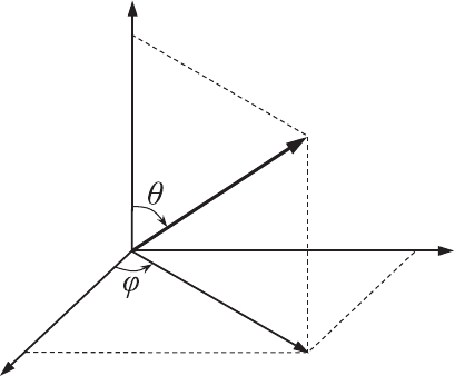
Problem 4.1. A free electron of mass m

, moves in the direction deﬁned by

the polar angle θ and the azimuthal angle ϕ (see Fig. 4.6). Find the electron

wavefunction (r, t) if the electron energy is equal to ε.

Problem 4.2. The dispersion equation Eq. (4.61) deﬁnes the allowed energy

states of an electron in a spherically-symmetric potential well and in a general

case it has to be solved numerically. Find the energy of stationary states in the

limit of inﬁnitely high potential barriers.

Problem 4.3. Find the energy levels and the wavefunctions of a positively

charged harmonic oscillator in a homogeneous electric ﬁeld E. The charge of

the oscillating particle is e and its mass is m.

Figure 4.6 Momentum p

in a spherical system of

coordinates.

4.6 Problems 135

Problem 4.4. An electron is in its ground state in a cubic potential well with

impenetrable barriers. Find the length, L, of the edge of the conﬁning cube and

the energy of the electron if the electron’s highest probability density is equal to

Problem 4.5. An electron is in its ground state in a cubic potential well

with impenetrable barriers and with edge length L =5 nm. Estimate the

pressure which the electron puts on the walls of the potential well. (Answer:

P = 0.35 × 10

Pa.)

Problem 4.6. At instant t = 0 the electron behavior is described by the following

wavefunction:

(r, 0) = Ae

−r

/α

+ikr

. (4.157)

Find the normalization constant, A, the most probable value r

, and the radial

part of the probability current, j.

Problem 4.7. An electron is in an inﬁnitely deep spherically-symmetric potential

well, i.e., U (r) = 0atr ≤ r

and U(r) =∞at r > r

, where r

is the radius

of the well. Find the form of the radial electron function, the electron energy in

s-states (l = 0), the magnitudes





and r



r

, the most probable value

, and the probability of the electron being in the region r ≤ r

Problem 4.8. For an electron in an inﬁnitely deep spherically-symmetric

potential well, i.e., U(r) = 0atr ≤ r

and U (r) =∞at r > r

, where r

is the

radius of the well, ﬁnd the dispersion equation for s-states in the energy region

E < U

and interval of values of U

when the well contains only one electron

energy level.

Problem 4.9. The wavefunction of the ground state of a one-dimensional har-

monic oscillator (particle with mass m in a one-dimensional parabolic potential

U (x) = mω

/2) has the following form:

ψ(x) = Ae

−bx

. (4.158)

Solve the Schr

odinger equation and ﬁnd the constant b and the energy of the

oscillator in the ground state.

Problem 4.10. The wavefunction of the one-dimensional harmonic oscillator in

a particular state has the following form:

ψ(x) = Axe

−bx

. (4.159)

Find the constant b and the energy of an oscillator in this state.

Problem 4.11. A particle with mass m moves in a three-dimensional parabolic

potential U (r) = mω

/2. Find the dependence of the oscillator’s energy on

the orbital quantum number.

Chapter 5

Approximate methods of ﬁnding

quantum states

The solution of most problems associated with electron quantum states in phys-

ical systems and structures (atoms, molecules, quantum nanostructure objects,

and crystals) is hard to ﬁnd because of the mathematical difﬁculties of getting

exact solutions of the Schr

odinger equation. Therefore, approximate methods of

solving such problems are of special interest. We will consider some of these

methods, such as the adiabatic approximation now and later the effective-mass

method, using real physical systems as examples. In this chapter we will consider

several widely used approximation methods for ﬁnding the wavefunctions and

energies of quantum states as well as the probabilities of transitions between

quantum states. First of all, we will consider stationary and non-stationary per-

turbation theories. What is common to these two theories is that it is assumed that

the perturbation is weak and that it changes negligibly the state of the unperturbed

system. Stationary perturbation theory is used for the approximate description of

a system’s behavior if the Hamiltonian of the quantum system being considered

does not directly depend on time. In the opposite case, non-stationary theory

is used. Then, we will brieﬂy consider the quasiclassical approximation, which

is used for the problems of quantum mechanics which are close to analogous

problems of classical mechanics.

5.1 Stationary perturbation theory for a system

with non-degenerate states

This theory is used for the approximate calculation of the energy levels and the

wavefunctions of stationary states of systems that are subjected to the inﬂuence

of small perturbations. Let us assume that the Hamiltonian of the quantum system

may be expressed in the following form:

H =

V , (5.1)

where

is the Hamiltonian of the unperturbed system and

V is the perturba-

tion operator. For the unperturbed Hamiltonian the solution of the Schr

odinger

136

5.1 Stationary perturbation theory, non-degenerate states 137

equation,

(0)

= E

(0)

, (5.2)

is assumed to be known, i.e., the complete set of eigenfunctions ψ

(0)

and eigen-

values E

(0)

of the unperturbed system is given. Let us assume, ﬁrst, that the unper-

turbed Hamiltonian,

, has a discrete spectrum and all states are non-degenerate.

This means that each eigenvalue E

(0)

corresponds to only one eigenfunction ψ

(0)

The complete set of these functions is orthonormalized, i.e., unperturbed wave-

functions satisfy the condition (2.144):



(0)∗

(0)

dV = δ

. (5.3)

It is necessary to ﬁnd the eigenvalues E

and the eigenfunctions ψ

of the

operator

H, i.e., the solutions of the following Schr

odinger equation:





= E

. (5.4)

This equation differs from Eq. (5.2)bytheterm

V ψ

, which is assumed to be

small in comparison with

, i.e., the state of the system must not change

considerably as a result of perturbation.

LetuslookforasolutionofEq.(5.4) in the form of a series expansion using

the complete set of eigenfunctions of the unperturbed Hamiltonian,



(0)

. (5.5)

Let us substitute this solution into Eq. (5.4) and use the fact that ψ

(0)

are the

eigenfunctions of the unperturbed Hamiltonian,

. As a result we get





(0)



(0)



(0)

. (5.6)

Let us multiply both parts of this equation by ψ

(0)∗

and integrate it over the entire

volume available for the quantum system:





− E

(0)





(0)∗

(0)

dV =





(0)∗

V ψ

(0)

dV. (5.7)

Taking into account the orthogonality condition (5.3), we arrive at the following

expression:





− E

(0)





, (5.8)

where V

is the matrix element of the perturbation operator

V , in the basis of

the unperturbed wavefunctions, ψ

(0)



(0)∗

V ψ

(0)

dV. (5.9)

138 Approximate methods of ﬁnding quantum states

The important feature of the Kronecker delta, δ

, is that it allows us to reduce

the number of indices in the summation. Taking into account the property of the

Kronecker delta, Eq. (5.8) reduces to



− E

(0)





. (5.10)

Equation (5.10) constitutes a system of linear algebraic equations for the unknown

coefﬁcients C

. This system is identical to the initial equation (5.4) since the

set of coefﬁcients C

completely deﬁnes the wavefunction (5.5). Finding the

exact solution of the system of Eqs. (5.10) is not much simpler than ﬁnding

the solution of Eq. (5.4). However, the system of Eqs. (5.10) can be solved

approximately using a series expansion over some small parameter. Let us present

the perturbation operator,

V ,intheform

V = 

W . (5.11)

Here,  is a small dimensionless parameter and

W is some perturbation operator.

Using the fact that  is small, we can present E

and C

in the form of a series

over the small parameter :

= E

(0)

+  E

(1)

+ 

(2)

+···, (5.12)

= C

(0)

+ C

(1)

+ 

(2)

+···. (5.13)

Here the magnitudes  E

(1)

and C

(1)

are of the same order as the perturbation

V , and the magnitudes 

(2)

and 

(2)

are of the second order of smallness,

i.e., the order of smallness is

,etc.

On substituting Eqs. (5.12) and (5.13)into(5.10) we get



(0)

− E

(0)



(0)

+ 



(0)

− E

(0)



(1)

+  E

(1)

(0)

+ 

(2)

(0)

+···

= 



(0)

+ 



(1)

+···. (5.14)

Let us ﬁnd the corrections to the energy E

(0)

and to the wavefunction ψ

(0)

for

the nth quantum state of the system. Since in the zeroth approximation ψ

= ψ

(0)

there is only one term in Eq. (5.14) that does not depend on , and it follows

that C

(0)

= 1 and all other coefﬁcients are equal to zero, C

(0)

= 0. Let us now

consider separately equations for k = n and k = n.Fork = n there is one term

on the left-hand side and one term on the right-hand side of Eq. (5.14)ofthe

ﬁrst order of smallness, i.e., proportional to . As a result, in the ﬁrst order of

approximation the correction to the energy E

(0)

is deﬁned as

 E

(1)

= W

= V



(0)∗

V ψ

(0)

dV =





, (5.15)

which is the average value of perturbation calculated using the corresponding

unperturbed state. Let us note that V

are usually called the diagonal matrix

elements of the perturbation operator,

V. For k = n from Eq. (5.14) it follows

5.1 Stationary perturbation theory, non-degenerate states 139

that

C

(1)

(0)

− E

(0)

, (5.16)

where the non-diagonal matrix elements of the perturbation operator, V

,are

deﬁned as



(0)∗

V ψ

(0)

dV, (5.17)

and C

(1)

= 0. Then, the corrections to the wavefunction in the ﬁrst order of

approximation are

(1)



n=k

(0)

− E

(0)

. (5.18)

To ﬁnd the corrections to the energy for the second order of approximation, we

equate the terms proportional to 

on both sides of Eq. (5.14). As a result the

correction E

(2)

is deﬁned as



(2)



n=k

(0)

− E

(0)

. (5.19)

As a rule, for the perturbed wavefunction it is sufﬁcient to determine the ﬁrst two

terms of the expansion and for the energy, the ﬁrst three terms of the expansion

of these magnitudes. As a result the wavefunction and the energy of the nth

perturbed state can be written as

= ψ

(0)



n=k

(0)

− E

(0)

, (5.20)

= E

(0)







n=k

(0)

− E

(0)

. (5.21)

These expressions are justiﬁed only when the next term of the expansion is

considerably smaller than the previous one. This condition is satisﬁed if the

matrix elements of the perturbation operator are considerably smaller than the

distance between the unperturbed levels, i.e.,





(0)

− E

(0)



, n = k. (5.22)

Example 5.1. An electron is conﬁned in a one-dimensional potential well with

inﬁnite-height barriers of width L and is affected by a perturbation, which has

the following coordinate dependence:

V (x ) = V

cos



π x



. (5.23)

Find the change of electron energy levels in the potential well using the second-

order approximation of the perturbation theory. Find the condition of applicability

of the perturbation theory in the case considered here.

140 Approximate methods of ﬁnding quantum states

Reasoning. Let us ﬁnd the matrix elements of the perturbation operator

V (x)

using the wavefunctions deﬁned by Eq. (3.51),

(0)

(x ) =



sin



nπ x



of the unperturbed problem:



(0)∗

V (x )ψ

(0)

dx =



cos



π x



sin



nπ x



sin



kπ x



dx.

(5.24)

As a result of integration we obtain for the matrix elements, V

,thefollowing

expression:











1, n = k = 1,

2, n = k = 1,

1, n = k ± 2,

0, n and k are other than the above.

(5.25)

The ﬁrst-order correction with regard to energy is equal to  E

(1)

= V

, and as

follows from Eq. (5.25), in the case when n = k = 1 we get

 E

(1)

= V

. (5.26)

In the case when n = k = 1 we get

 E

(1)

= V

. (5.27)

Taking into account Eq. (5.25), the second-order correction, deﬁned according

by Eq. (5.19), is equal to



(2)



n=k

(0)

− E

(0)

=−

64π







1, n = 1,

2/3, n = 2,

−4/[(n + 1)(n − 1)], n ≥ 3,

(5.28)

where E

(0)

is deﬁned by Eq. (3.44):

(0)

In deriving Eq. (5.28) we took into account that for n = k only V

with n = k ±

2 are not equal to zero. The condition of applicability of the perturbation theory

(5.22) in the current problem taking into account the unperturbed eigenvalues of

energy (Eq. (3.44)) reduces to the following inequality:



2π

(

n − 1

)

. (5.29)

5.2 Stationary perturbation theory, degenerate states 141

5.2 Stationary perturbation theory for a system

with degenerate states

Very often we deal with degenerate states of an unperturbed quantum system.

Let us assume that the eigenvalues of the unperturbed Hamiltonian,

,are

degenerate and that the order of degeneracy of the nth energy level, E

(0)

,is

equal to s. In this case s orthogonal wavefunctions ψ

(0)

,...,ψ

(0)

correspond to a

single eigenvalue E

(0)

. The perturbation splits the degenerate energy level, E

(0)

into s closely spaced sublevels. Each of the sublevels is described by its own

wavefunction, which is a linear combination of the unperturbed wavefunctions

(0)

. Let us assume that the perturbation

V is small. Therefore, we are expecting

closely spaced energy levels in the ﬁrst order of approximation of perturbation

theory.

Let us consider the case of a doubly degenerate energy level E

(0)

with corre-

sponding eigenfunctions, ψ

(0)

and ψ

(0)

. The wavefunction of the perturbed state,

, can be written as a superposition of unperturbed wavefunctions:

= C

(0)

+ C

(0)

. (5.30)

After the substitution of ψ

into Eq. (5.4), multiplication of Eq. (5.4)bythe

complex-conjugate function ψ

∗

, and its integration (as we did in the previous

section), we get the following system of algebraic equations with the unknown

coefﬁcients C

and C



(0)

+ V

− E



+ V

= 0,



(0)

+ V

− E



= 0,

(5.31)

where the matrix elements of the perturbation operator are deﬁned by Eq. (5.17):



(0)∗

V ψ

(0)

dV. (5.32)

Non-zero solutions for C

and C

exist only in the case when the determinant of

the system of Eqs. (5.31) equals zero. By equating the determinant to zero we

obtain the following quadratic equation with respect to energy E

−



(0)

+ V





(0)

+ V



(0)

+ V



− V

= 0. (5.33)

The solution of this equation can be written as

= E

(0)

+ E

(1±)

, (5.34)

where the corrections of the ﬁrst order E

(1±)

to the unperturbed energy state E

(0)

are deﬁned by the expression

(1±)

+ V



− V

)

+|V

, (5.35)

142 Approximate methods of ﬁnding quantum states

and V

=|V

. The sign “±” in Eq. (5.35) indicates that in the presence of

perturbation the degeneracy of the unperturbed quantum system is lifted and the

energy levels split into two sublevels.

On substituting the expressions for the energy into the system of Eqs. (5.31)

we get for the coefﬁcients of expansion the following relation:

= C

− E

(0)

− V

≡ C

− E

(0)

− V

. (5.36)

In a system of homogeneous linear algebraic equations such as Eq. (5.31) one

of the coefﬁcients is always arbitrary. In our case we take the coefﬁcient C

arbitrary. We will ﬁnd C

later, from the normalization condition of the wave-

function ψ

. Taking into account the normalization and orthogonality conditions

of the unperturbed wavefunctions, ψ

(0)

and ψ

(0)

, the normalization condition of

the wavefunction ψ

takes the form

+|C

= 1. (5.37)

On substituting Eq. (5.36) into Eq. (5.37) we obtain the following expressions

for the expansion coefﬁcients C

and C



2|V



1 ±

− V



− V

)

+ 4|V



1/2

, (5.38)

∓



2|V



1 ∓

− V



− V

)

+ 4|V



1/2

. (5.39)

Thus, in the case of doubly degenerate states the corresponding energy level

splits into two sublevels, which correspond to the following wavefunctions:

= C

(0)

∓

(0)

. (5.40)

5.3 Non-stationary perturbation theory

Very often it is necessary to solve problems in which the perturbation which

acts on the quantum-mechanical system depends on time. Let us assume that

the initial state of a quantum system is a stationary state. It is necessary to ﬁnd

the state of the system at a later time t if at the initial instant, t = 0, the small

perturbation, which depends on time, begins to act. In this case the ﬁrst term,

, in the Hamiltonian of the quantum system (5.1) does not depend on time,

while the perturbation,

V (t), depends on time. We have to ﬁnd the change of the

system’s state with time. Generally this can be described by the non-stationary

Schr

odinger equation



(0)

V (t)



(x, t) = ih

∂(x, t)

∂t

. (5.41)