Navarra Antonio, Simoncini Valeria. A Guide to Empirical Orthogonal Functions for Climate Data Analysis

Подождите немного. Документ загружается.

6.2 Cross-Covariance Analysis Using the SVD 99

would not be pairwise orthogonal. Generic matrices of this kind are difﬁcult to treat

and they appear to have no particular properties that can be exploited to our aims.

However, in this situation we can probably fully appreciate the power of the results

presented in Chap. 2 regarding the Singular Value Decomposition. Any matrix can

in fact be decomposed with an SVD. In our case we can apply the SVD to the cross-

correlation matrix,



D U†V



: (6.3)

The orthogonal matrices composed of the column vectors u’s and v’s, U D

; u

;:::;u

/, V D .v

; v

;:::;v

/ yield bases in the Z and S data ﬁelds,

respectively, and the modes are paired, sharing the same singular values. The ﬁelds

can be reconstructed using the columns of U; V with

iD1

; z

and s

iD1

: (6.4)

We can give an interpretation of the singular values and modes that is similar to

the EOF: the decomposition corresponds to saying that the total cross-covariance is

given by the singular value sum. The ratio of each singular value can be interpreted

as the fraction of cross-covariance that can be attributed to that particular mode, as

in the following relation:





iD1



: (6.5)

6.2 Cross-Covariance Analysis Using the SVD

The cross-covariance seems a natural extension of the concept of the covariance (the

autocovariance)that we have discussed in the previous chapters. It is then reasonable

to wander whether it is possible to extend the concept of EOF to the more general

case. We have to resort to the general idea that the EOF are the directions, in the data

space, that explain most of the cross-covariance. We may ask to look for a similar

pattern that performs the same role. It is easy to see that if we choose the basis of

the left and right singular vectors deﬁned in the preceding section we can get indeed

what we are looking for. With (6.4) in mind, we expand the data over the right and

left singular vectors, obtaining two matrices of expansion coefﬁcients, A and B,that

represent the data in the new bases formed by the singular vectors,

Z D UA; S D VB:

The cross-correlation matrix has a very simple form in this basis, namely

100 6 Cross-Covariance and the Singular Value Decomposition

D UA.VB/

D UAB

Comparing this decomposition with that in (6.3), it follows that it must be

† D AB

: (6.6)

This means that the basis of the singular vectors of the cross-covariance matrix

is such that the matrix itself is diagonal. It can also be shown that the diagonal val-

ues on the left-hand side of (6.6) are the values of the time series covariance of

the singular vectors coefﬁcient and that such covariances are maximized. Therefore,

the singular vectors represent patterns with maximum covariances between the time

series. They diagonalize the cross-covariance matrix in the same way the EOF diag-

onalize the covariance matrix, yielding a special basis of unconnected patterns. The

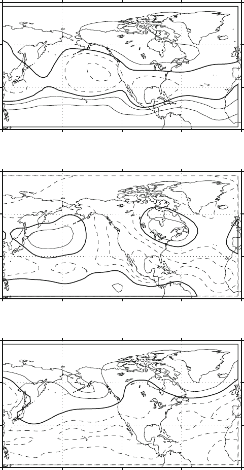
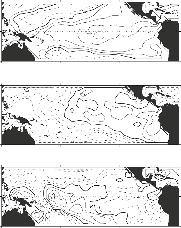
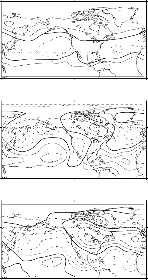
following pictures show the result of this analysis when it is applied to the already

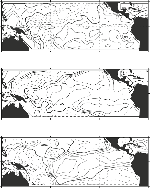
introduced height and SST ﬁelds. Figure 6.1 shows the patterns for the Z component

of the SVD analysis, whereas Fig. 6.2 shows the SST component.

The interpretation of the explained variance needs some discussion. The “diag-

onalization” of the cross-covariance matrix indicates that it is possible to interpret

the diagonal singular values as the contribution to the total cross-covariance for that

particular mode, in case we deﬁne the total cross-covariance as the trace of the ma-

trix † , namely the sum of the singular values. The modes can be ranked according

to the amount of explained cross-covariance (CC) as it is represented in Figs 6.1

and 6.2. The amount is the same for the separate component of the mode. However,

when we consider the mode components as a basis for the height or the SST, there

is no guarantee that any relation exists between the relative importance of the two

modes and it is possible that we get different amount of variance explained by the

two factors. The amount of total variance explained by the two components when

they are considered separately (TC) is also shown in the pictures. In some cases they

are similar and in others different, there is no relation that forces a particular amount

of explained variance.

The patterns themselves show some resemblance to the pattern of the EOF of

the height ﬁeld (Fig. 4.8) and to the Combined EOF (Fig. 5.13). This is not too

surprising, since we are dissecting the same variability, each time trying to stress

different aspects of it. The difference is larger when we go to higher modes, as it

should be expected.

As in the case of the EOF, the analysis yields patterns that are idealizations, in

the sense that they do not represent any physically realized pattern, but patterns

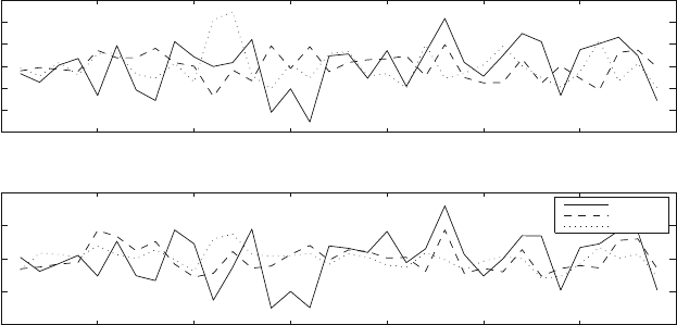
that correspond to an optimization criterion for the cross-covariance. The SVD has

identiﬁed patterns of covariation between the two different ﬁelds, as it can be seen

from the inspection of the time series of the coefﬁcients (Fig. 6.3).

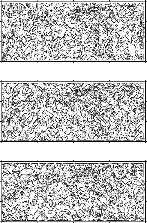
It is possible to have a measure of the method’s ability to capture the covariations,

by applying it to a data set of randomly chosen data. Figure 6.4 shows the result

when the cross-covariance SVD method is applied to a random data set of the same

dimension in time and space of the previous pictures. The random nature of the

cross-covariance is very well expressed by the absence of any structure, in the sense

6.2 Cross-Covariance Analysis Using the SVD 101

−0.06

−0.06 0.040.04

0.04

SVD Z Component Expl TC 33% Expl CC 84%

−0.06

SVD Z Component Expl TC 9% Expl CC 5%

SVD Z Component Expl TC 18% Expl CC 4%

−0.06

0.04

90°N

60°N

30°N

0°

90°N

60°N

30°N

0°

90°N

60°N

30°N

0°

120°E 180°W 120°W 60°W 0°

Fig. 6.1 The ﬁrst three SVD modes for the Height-SST data set. Here is shown the Z component

in descending order of explained total combined variance

102 6 Cross-Covariance and the Singular Value Decomposition

−0.06

60.0−60.0−

0.04

−0.06

0.04

S Component Expl TC 33% Expl CC 84%SVD

S Component Expl TC 10% Expl CC 5%SVD

−0.06

0.04

−0.06

0.04

−0.06

0.04

−0.06

0.04

−0.06

0.04

S Component Expl TC 5% Expl CC 4%SVD

180°W

120°E

60°W120°W

180°W

120°E

60°W120°W

180°W

120°E

60°W

120°W

30°N

30°S

0°

30°N

30°S

0°

30°N

30°S

0°

Fig. 6.2 The ﬁrst three SVD modes for the Height-SST data set. Here is shown the SST component

in descending order of explained total combined variance

of organized, large scale features, in the pattern spatial distribution. The patterns

are indeed casual, indicating that the SVD is trying to do its best at optimizing

the little cross-covariance occurring in the random data, but with limited success,

since the amount of cross-covariance explained (TC) is very small, as the amount of

total variance explained (CC) is also small. The cross-covariance is in fact almost

6.2 Cross-Covariance Analysis Using the SVD 103

0 5 10 15 20 25 30 35

−60

−40

–20

Time series of the first three SVD modes −− Z component

0 5 10 15 20 25 30 35

−40

−20

Time series of the first three SVD modes −− S component

Mode 1

Mode 2

Mode 3

Fig. 6.3 The time series coefﬁcients for the ﬁrst three SVD modes for the Height-SST data set

uniformly distributed among the modes, a symptom of the data randomness and of

the absence of any relation between the two ﬁelds.

Another interesting insight can be obtained by repeating the SVD analysis be-

tween the height and SST ﬁelds, but this time we rearrange the time series of the

SST in a random way, so that we possibly destroy the relation in time that is the tar-

get of the SVD analysis. The permutation has been selected in such a way to reduce

by 50% the amount of total cross-covariances between the two ﬁelds. It is totally

arbitrary, so that months in Z in different years can be paired to different months of

the SST. The results are shown in Figs. 6.5 and 6.6. The patterns do not show any

particular deﬁciency and in fact they could be plausible patterns. They exhibit the

kind of structure that can be considered typical of the variability of these ﬁelds, as

we have seen in the various analyses so far. The SVD aims at emphasizing patterns

that satisfy the optimization requirement even in presence of weak (by construc-

tion) cross-relation. Nevertheless the patterns themselves are plausible because they

bring the signature of the internal variability (namely the individual covariance) of

the ﬁelds so as not to get crazy patterns as in the previous example of the completely

random ﬁelds.

This example shows one of the most insidious pitfalls of this kind of analysis. The

mathematical requirements, the optimization criterion, the orthogonality constraint

etc., can force structure even when it is unlikely to exist. In a real case, with no a

priori knowledge of what structure to expect, there is a problem on how to assess the

reliability of the structures found by the SVD and of the implicit covariant relations

found. Actually, maybe some warning could be found in the small portion of total

variance explained by the modes found by the SVD (see the TC values in the ﬁgures)

that are in any case cautioning towards attributing an excessive importance to the

structures.

104 6 Cross-Covariance and the Singular Value Decomposition

−0.06

−0.06−0.06

SVD Z Component Expl TC 3% Expl CC 4%

−0.06

−0.06−0.06

SVD Z Component Expl TC 3% Expl CC 4%

−0.06

−0.06−0.06

0.04

SVD Z Component Expl TC 3% Expl CC 4%

120°E 180°W 120°W 60°W 0°

90°N

60°N

30°N

0°

90°N

60°N

30°N

0°

90°N

60°N

30°N

0°

Fig. 6.4 The ﬁrst three SVD modes for a randomly chosen left and right ﬁeld data set. Here is

shown the Z component in descending order of explained total combined variance

6.2 Cross-Covariance Analysis Using the SVD 105

−0.06

0.04

SVD Z Component Expl TC 34% Expl CC 32%

−0.06

0.04

SVD Z Component Expl TC 8% Expl CC 21%

−0.06

−0.06−0.06

0.04

−0.06

SVD Z Component Expl TC 6% Expl CC 13%

120°E 180°W 120°W 60°W 0°

90°N

60°N

30°N

0°

90°N

60°N

30°N

0°

90°N

60°N

30°N

0°

Fig. 6.5 The ﬁrst three SVD modes for the height and a randomly permuted SST data set. Here is

shown the Z component in descending order of explained total combined variance

106 6 Cross-Covariance and the Singular Value Decomposition

−0.06

60.0−60.0−60.0−

0.04

−0.06

0.04

S Component Expl TC 7% Expl CC 32%SVD

−0.06

0.04

0.040.04

0.04

−0.06

0.04

S Component Expl TC 22% Expl CC 21%SVD

−0.06

0.04

−0.06

S Component Expl TC 12% Expl CC 13%SVD

30°N

30°S

0°

30°N

30°S

0°

30°N

30°S

0°

180°W

120°E

60°W120°W

180°W

120°E

60°W120°W

180°W

120°E

60°W120°W

Fig. 6.6 As in Fig. 6.5 but for the SST modes

Chapter 7

The Canonical Correlation Analysis

7.1 The Classical Canonical Correlation Analysis

The method based on the Singular Value Decomposition described in previous

chapters was able to represent the largest amount of cross-covariance with fewest

modes. The computed modes are designed so as to speciﬁcally explain most of

the spatial variance. The spatial view point is a requirement that can be put on the

modes, but it is hardly unique. Another commonly employed point of view arises if

one considers the temporal variations of the modes. In this case one is interested in

modes that generate maximally correlated time coefﬁcients. This method has been

developed in multi-variate analysis and it is known as “Canonical Correlation Anal-

ysis”. In mathematical terms we seek a decomposition of the data matrices such that

the time coefﬁcients are deﬁned as

iD1

; and s

iD1

;

where u; v are unknown patterns and a; b are the time coefﬁcients, so that the entire

ﬁelds can be reconstructed. We require that the coefﬁcients taken as a time series

are uncorrelated with each other,

D ı

;

where ı

satisﬁes ı

D 0 for k ¤ l and ı

D 1, and the angular bracket denotes

the scalar product (or correlation operation). The spatial ﬁelds u and v are to be

determined as those particular spatial distributions that enforce orthogonality of the

time coefﬁcients. Assuming Z and S of full row rank, the solution to the problem can

be formally obtained by computing an SVD on a normalized version of the cross-

covariance matrix. In the following we ﬁrst reproduce the classical description of the

procedure, and then present a computationally more elegant and sound approach that

yields a mathematically equivalent solution. We write the SVD on the normalized

matrices as

.ZZ







.SS





D U†V



: (7.1)

A. Navarra and V. Simoncini, A Guide to Empirical Orthogonal Functions

for Climate Data Analysis, DOI 10.1007/978-90-481-3702-2

 Springer Science+Business Media B.V. 2010

107

108 7 The Canonical Correlation Analysis

The left and right singular vectors cannot be used directly to reconstruct the original

data matrix, they must be scaled to obtain the so-called “weight vectors”

WD .ZZ





U; W

WD .SS





V: (7.2)

The weight vectors, that is the columns of W

and W

, can be used to derive the

time coefﬁcients for the reconstruction of the synthesized data set, a

;

, or in matrix notation,

A D Z



; B D S



: (7.3)

The matrices A and B have orthonormal columns (corresponding to time). Indeed,



A D W



D U



.ZZ







.ZZ





U D I: (7.4)

A similar result holds for B. The cross-product of A and B yields an interesting

result:



B D W



D U



.ZZ







.SS





V D U



U†V



V D †; (7.5)

where we have used (7.1) and the orthogonality propertyof the left and right singular

vectors in the second line. The cross-correlation in time between the coefﬁcients of

the same modes is then a measure of the singular values of the cross-covariance

matrix scaled as in (7.1).

In practice, the explicit computation of the inverse square roots in (7.1)isavoided

by ﬁrst computing the SVD of the two matrices Z and S.Let

Z D U

†



; S D U

†



(7.6)

be the so-called “economy size” SVD of Z and S, respectively.

Therefore,

.ZZ





Z D U

.†

†







†



D U



;

where

is the matrix containing the ﬁrst columns of V

, so as to match the size

of U

. Here we have used the fact that †

D Œdiag.

;:::;

/; O. An analogous

derivation follows for S. Hence







.SS





D U



Computing the SVD of this latter matrix, that is



D U†V



; so that



D U



U†V



;

The term “economy size” in the factorization U†V



refers to the fact that only the columns of U

and V corresponding to nonzero diagonal elements in † are retained. Therefore, assuming that the

given matrix has maximum rank, either U or V is rectangular.