Navarra Antonio, Simoncini Valeria. A Guide to Empirical Orthogonal Functions for Climate Data Analysis

Подождите немного. Документ загружается.

7.3 The Barnett–Preisendorfer Canonical Correlation Analysis 119

Chap. 4 can be used to deﬁne a criterion to choose a number of EOF to keep. The

sensitivity of the BP-CCA method is however smaller (Fig. 7.6). We can see in Figs.

7.7 and 7.8 that the ﬁrst mode is not much affected by the changes in the amount

of variance retained in the BP-CCA analysis. The second mode is more sensitive,

showing marked differences according to the number of EOF kept in the original

data sets.

0.96959

0.969592

60N

90N

120W 60W

30N

120E 180E

Z Component 50% Expl TC 12% Correlation 92%

First Mode

CCA−BP

−0.879728

60N

90N

120W 60W

30N

120E 180E

Z Component 80% Expl TC 12% Correlation 97%

120W 60W120E 180E

−0.974662

60N

90N

30N

Z Component 90% Expl TC 13% Correlation 98%

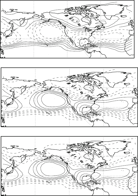
Fig. 7.7 The ﬁrst CCA Barnett–Preisendorfer mode for the Height-SST data set. Here is shown

the Z component for different numbers of retained EOF. The EOF retained correspond to keeping

50%, 80% and 90% of the variance, respectively

120 7 The Canonical Correlation Analysis

1.6764

60N

90N

120W 60W

30N

120E 180E

Z Component 50% Expl TC 9% Correlation 9%

Second Mode

CCA−BP

120W 60W120E 180E

−1.7531

60N

90N

30N

Z Component 80% Expl TC 1% Correlation 84%

120W 60W120E 180E

60N

90N

30N

−1.5537

Z Component 90% Expl TC 1% Correlation 95%

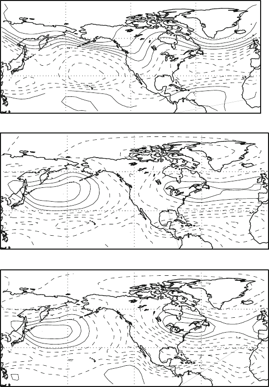
Fig. 7.8 The second CCA Barnett–Preisendorfer mode for the Height-SST data set. Here is shown

the Z component for different numbers of retained EOF. The EOF retained correspond to keeping

50%, 80% and 90% of the variance, respectively

The direct comparison is made difﬁcult by the uncertainty in the sign that the

CCA modes share with the other methods. Weight vectors and patterns are deter-

mined up to a an overall sign by CCA, either in the original version or according

to the BP prescription. This means that the algorithm used to compute the modes

7.3 The Barnett–Preisendorfer Canonical Correlation Analysis 121

randomly picks one sign. General consistency is guaranteed by the fact that the co-

efﬁcients sign is changed accordingly. This is easy to recognize in the patterns, but

it may become tricky if time series from different calculation are compared. Care

must be taken to make sure that the modes are comparable in terms of having all

the same sign convention. The strategies used to choose an appropriate sign for the

EOF (see Chap. 4) can also be employed here.

Chapter 8

Multiple Linear Regression Methods

8.1 Introduction

In the previous chapters we have introduced techniques to ﬁnd relations between

two or more different ﬁelds. In this chapter we describe a more general framework

that may provide additional insight into previously analyzed methods. In general a

relation between ﬁelds can be formulated symbolically as

Z D f.S/ (8.1)

where, for instance, Z represents the geopotential and S the SST. The exact form

of the relation is unknown, but it is probably time dependent and thus includes

effects of time lags and so on. In practice, it is really difﬁcult to investigate arbitrary

functional forms for f in (8.1); assuming f to be linear represents a simplifying

but viable alternative. In this case the function f may be represented by matrices.

We have seen in the previous chapters that powerful methods have been devised

to identify relations of the form (8.1) assuming that f.S/ is a linear function. We

have seen linear correlation methods, teleconnection analysis and ﬁnally methods

that analyze systematically the linear relation between two data sets, such as the

Singular Value Decomposition (SVD) or Canonical Correlation Analysis (CCA).

We will now deﬁne a general framework that includes the latter as special case.

Assuming linearity, the relation between the data matrices Z and S can be written

as (Navarra and Tribbia 2005)

Z D AS (8.2)

where A is a matrix, assumed here to be stationary. Z and S are data matrices de-

scribing the atmospheric and oceanic ﬁelds arranged at ﬁxed times. In general, the

number of spatial points need not be the same in the Z and S data and so the two ma-

trices will be in general rectangular matrices, with n time columns and, respectively,

p rows for Z and q rows for S.

It is possible to set a simple (least squares) minimization problem for A (Golub

and Van Loan 1996; Richman and Vermette 1993), as

A. Navarra and V. Simoncini, A Guide to Empirical Orthogonal Functions

for Climate Data Analysis, DOI 10.1007/978-90-481-3702-2

 Springer Science+Business Media B.V. 2010

123

124 8 Multiple Linear Regression Methods

min

Z AS

(8.3)

where the norm is the Frobenius norm, as deﬁned in (2.5). If SS

is full rank, the

minimizing least squares solution can be written as

A D ZS

.SS

1

: (8.4)

If S is square, the solution is exact and the residual Z AS is zero. Otherwise the

obtained solution minimizes the residual among all possible choices of A, yielding

a nonzero residual. If SS

is singular, then a solution can still be found by using the

pseudoinverse deﬁned in (2.12).

The matrix A in (8.4) describes the relation between the ﬁelds S and Z, and it is

the operation that transforms the S ﬁeld into Z.

In the case that the minimum is zero, then the entire ﬁeld Z can be transformed

into S. In this case AS D Z and the range of A spans the whole space Z. In addition,

the variances of AS and of Z coincide, namely

diag..AS/.AS/

/ D diag.ZZ

where we recall that we are still assuming that the ﬁelds have zero mean.

If the minimum is not zero, then AS does not coincide with the space Z and in

general the range of A will be a subspace of Z. Now only a portion of the ﬁeld

Z’s variability can be associated with the variability of AS. There is a difference

between the ﬁeld Z and AS so that

free

D Z  AS:

In general we can thus write the ﬁeld Z as

Z D AS C Z

free

D Z

C Z

free

: (8.5)

This splitting of Z makes explicit that a portion of the ﬁeld Z can be reached

directly from S via the operator A (denoted by Z

), but a residual part, Z

free

, cannot

be reached. It is interesting to observe that the two parts are uncorrelated in time,

that is

free

D 0:

Indeed,

free

D Z

 S

/ D ASZ

 ASS

D ASZ

 ASS

.SS

1

D 0:

8.1 Introduction 125

Exercises and Problems

1. Given the matrices S D Œ1; 1; 1; 1I 1; 1; 1; 1I and Z D Œ1; 1; 2; 0I

0; 1; 1; 2I 0; 0; 1; 1, compute the least squares solution of the problem

min

kZ  ASk

We have

A D .ZS

/.SS

1

42





1

10:5

10:5

00:5

2. With the data of the previous exercise, verify that the residual is orthogonal to

AS.

A direct computation shows that

.AS/Z

free

3 131

1313

1111



111

1 1 1

1 11

111

D 0:

8.1.1 A Slight Digression

The search for a relation between the ﬁelds can also be formulated in a different

way, via the following minimization problem:

min

S BZ

;

where we are trying to get S in terms of Z. This problem has an analogous mini-

mization solution

B D SZ

.ZZ

1

: (8.6)

We now have two operators, A and B, that express the relation between S and

Z, but that are not completely equivalent. The operator A can be interpreted as

expressing the inﬂuence of S in terms of Z, whereas the operator B represents the

inﬂuence of Z on S. They both involve the cross-correlation matrix ZS

and its

transpose SZ

. In general there is no reason to expect them to have any special

structure.

Further insight can be gained by realizing that each of (8.4)and(8.6)representsa

multivariate regression problem for the atmospheric ﬁeld Z on the oceanic SST ﬁeld

S. This is a general formulation of the coupling problem, that is the identiﬁcation of

the relation between two varying ﬁelds. It is only subjected to the linearity constraint

126 8 Multiple Linear Regression Methods

in the coupling, and it will give an indication of the strength of the relation between

one ﬁeld and the other. The method based on the matrices A and B obtained via

the Least Squares method will be denoted in the following as the PRO method.

This is reminiscent of the name, PROcrustes problem, commonly employed for this

formulation in the climatology community, although the true Procrustes problem

requires additional constraints, and it is discussed in Sect. 8.2.2.

It is interesting to note that the method based on the pseudoinverse can be applied

to any pair of ﬁelds. We also have made no assumptions regarding the geographical

location of the data we are using for the analysis. The ﬁelds S and Z could be located

in the same geographical domain or they could be placed in remote locations distant

from each other. We might consider, for instance, the geopotential and the SST in the

same domain in the tropics, or we might take the tropical SST and the geopotential

over North America. In the former case we are looking at local relation between

the ﬁelds, in the latter case we are really looking at remote inﬂuences, probably

mediated by other physical processes.

8.2 A Practical PRO Method

The cost of the calculation described in the preceding section depends strongly on

the order of the data matrices. It is a function of the row and column dimension of

Z and S. The cross-correlation matrix ZS

, that is the essential part of A,mayhave

very large dimension if many grid points are considered. In our case, its dimensions

are p q. In some applications it is not a problem, but for a typical climate or mete-

orological application the number of grid points can quickly run into the thousand,

making the calculation of ZS

unpractical.

A signiﬁcant simpliﬁcation of the calculation can be achieved by using the data

compression properties of the EOF. Using the EOF we have introduced in previous

chapters we can achieve a signiﬁcant reduction in the problem size to be solved. The

maximum number of EOF for a data ﬁeld, say Z, is given by the smaller dimension

of Z. In typical meteorological applications the number of time levels is often much

smaller than the number of grid points and we can reduce the problem signiﬁcantly.

If the columns of U

, U

contain the EOFs of the two ﬁelds Z, S, respectively,

that is, their left singular vectors, then we know from Chap. 4 that

Z D U

Z; S D U

We can then deﬁne the signiﬁcantly smaller problem in terms of the EOF

coefﬁcients as

min

Z A

Its solution can be found in a similar way in terms of the tilde quantities as

A D

1

: (8.7)

8.2 A Practical PRO Method 127

The reduction of the algebraic dimension of the problem is quite signiﬁcant.

In the case of a geophysical ﬁeld, the data matrices are usually very rectangular,

because the number of columns describing the spatial extent of the ﬁeld is usually

much larger than the number of rows describing the number of time levels analyzed.

The minimization problem is then quite tractable. The use of EOFs also offers the

possibility of an interpretation of the operators A and B. The operator A expresses

the contribution to a single mode of Z, for instance the ﬁrst mode by all the modes

of S. By inspecting the columns of A we can analyze the regression factor by which

each mode of S contributes to that particular mode. Large values indicate a strong

impact of that S mode on the variability of the ﬁrst Z mode. The analysis can be

repeated for each column, thereby reconstructing the map of the S modes that have

strong inﬂuences on Z. A similar argument can be done for the operator B,inwhich

the role of S and Z are reversed. In this case the column will indicate which of the

Z modes contributed more strongly to the ﬁrst S mode. Together, the two operators

contain a fairly detailed map of the inﬂuence patterns between the ﬁelds.

The operator B can be interpreted in a similar way, with the role of Z and S

reversed. Now the (1,1) component of B expresses the inﬂuence of the ﬁrst Z mode

on the ﬁrst S mode or of the second mode on the ﬁrst mode, and so on.

In principle, the usage of the EOF allows one to ﬁlter the data prior to the appli-

cation of the PRO method, by retaining only some of the EOF and achieving another

signiﬁcant saving. This is not required by the method itself, but is a feature that adds

further ﬂexibility to the method and can be helpful in avoiding overﬁtting.

8.2.1 A Different Scaling

It is interesting to note what happens when the data are scaled by the covariance

matrices. If we take the data in the EOF representation and we scale them by the

square root of their covariance matrices,

Z D .



S D .



then

D I;

D I:

When this scaling is used the cross-covariance matrix becomes the cross-

correlation matrix. The minimizing solution to the scaled least squares problem

min

Z A

can then be written as

A D

128 8 Multiple Linear Regression Methods

Interestingly the sister problem can be solved as

B D

and so A D B

In this scaling the inﬂuence matrices A and B are one the transpose of the other.

This means that only one matrix is sufﬁcient to describe the interaction among the

various modes. In this case, the upper half of the matrix describes the inﬂuence of Z

on S and the lower half the inﬂuence of S on Z. This scaling is used in the Canonical

Correlation Analysis approach and this relation prompts us to examine what are

the connections between the PRO methods and the other methods used to analyze

variance.

8.2.2 The Relation Between the PRO Method and Other Methods

It is interesting to analyze what happens if further restrictions are put on the coupling

matrix A. If we require that A be an orthonormal matrix Q,i.e.QQ

D Q

Q D 1,

then we obtain the orthogonal Procrustes problem,

min

Z  QS

; (8.8)

whose solution is given by (see, e.g., Golub and Van Loan 1996, sec.12.4.1)

Q D UV

;

where U and V are obtained by the Singular Value Decomposition of the cross-

correlation matrix, that is

D U˙V

This is the deﬁnition of the SVD method as proposed by Bretherton et al. (1992),

and we can now see that it is essentially a Procrustes problem. This result is con-

sistent with Cherry (1996, 1997) who found that the SVD method essentially aims

at rotating one data set into the other. Searching coupled modes with SVD is there-

fore equivalent to assuming a priori that the coupling relation between the ﬁelds is

special. Similarly, it is also possible to realize that the Canonical Correlation Anal-

ysis imposes a similar orthogonality requirement on Q. From this point of view it is

The name is taken from the Greek mythology. Procrustes, the owner of a tavern, had only one

bed and therefore took to sawing off the legs of his guests if they were too long for his bed. In a

similar way, we are trying to “constrain” the matrix Z into S and we are willing to chop off some

part of Z in order to so.

8.3 The Forced Manifold 129

not surprising that identiﬁcation of coupled modes via SVD or CCA is sometimes

arduous, since the orthogonality constraint for the inﬂuence operators does not seem

to have any physical justiﬁcation.

8.3 The Forced Manifold

It is often the case in meteorology or climatology that numerical simulations are re-

peated with similar forcing conditions and slightly different initial conditions. The

reason can be found in the extremely sensitive nature of the atmospheric systems to

small perturbations in the initial values. Small initial differences can quickly evolve

in large differences because of the natural growth of instabilities and other nonlin-

ear feedbacks. This phenomenon makes sometimes difﬁcult the detection of signal

imposed on the climate systems by external factors, like for instance a certain pre-

scribed distribution of Sea Surface Temperatures (SST). In the preceding chapters

we have often used data from simulations that were derived exactly in that man-

ner, the objective to isolate the effect on the atmospheric variability of the changes

in SST. This kind of experiments is often designed as an ensemble experiment in

which the same SST distribution changing in time month after month is used and

several simulations with slightly different initial values are used. A number of sta-

tistical methods can then be used on the resulting ensembles to detect the effect of

SST.

We can use the PRO method described in the previous sections to extract the

signal from these experiments. The data matrix for Z must be extended to include

all the members of the ensemble

Z D Œz

; z

; :::; z

; z

; :::; z

; :::;

where the superscripts a;b;::: label the individual members of the ensemble. The

data matrix for S is obtained by repeating the time series to match the number of

members

S D Œs

; s

; :::; s

; s

; :::; s

; ::::

The PRO method can then be applied to the data matrices Z and S. Figure 8.1

shows the result of the PRO method when it is applied to the Paciﬁc North American

region for the atmospheric ﬁeld Z and to the tropical region for the SST. The PRO

method divides the ﬁeld Z in two orthogonal parts, the ﬁrst component has maxi-

mum correlation with the other ﬁeld, in this case the SST, the second is uncorrelated

from the SST. In mathematical terms the two parts are subspaces of the original

data, we can call them the Forced Manifold in the ﬁrst case, to represent the fact

that the subspace contains the effects of the forcing ﬁeld and we may call the other

Free Manifold to represent its independence of the variations of the forcing ﬁeld.

The ﬁgure shows the ratio between the variance of the Forced Manifold and the total

variance locally point by point. The orthogonality of the two subspaces can be seen