Navarra Antonio, Simoncini Valeria. A Guide to Empirical Orthogonal Functions for Climate Data Analysis

Подождите немного. Документ загружается.

130 8 Multiple Linear Regression Methods

Variance of Forced manifold for Z 44 %

00 0.10.1 0.20.3

0.3

0.40.4

0.4

0.5

0.6

0.7

0.6

0.5

0.6

0.4

0.5

0.3

0.7

0.6

60W120W180W120E

30N

60N

90N

Variance of Free manifold for Z 56 %

00 0.10.1 0.20.2

0.3

0.4

0.5

0.6

0.7

0.5

0.4

0.3

0.8

0.5

0.6

0.7

0.4

60W120W180W120E

30N

60N

90N

Variance of S

0.1

0.2

0.3

0.4

0.5

0.6

0.7

0.1

0.8

0.1

0.9

0.1

0.2

0.1

0.9

60W120W180W120E

20S

10S

10N

20N

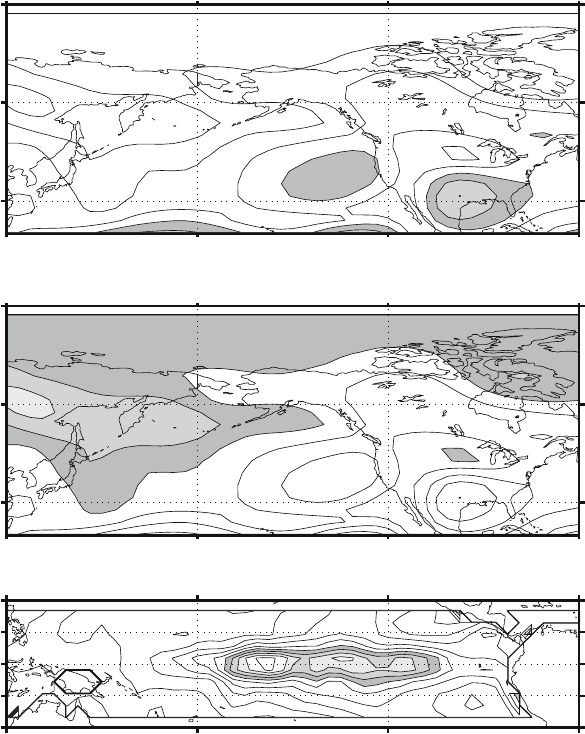
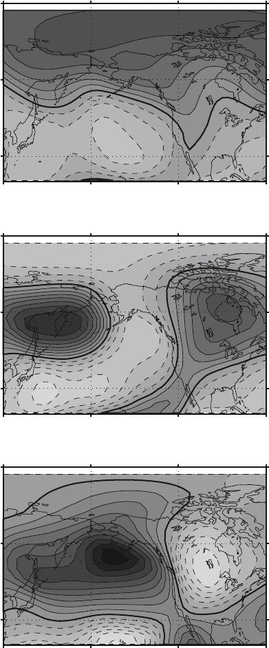
Fig. 8.1 Forced Manifold and Free Manifold. The picture represents the division in Forced and

Free Manifold for the North American geopotential ﬁeld Z in the region north of 20N and the

tropical Paciﬁc SST in the region 20N–20S latitude. The top panel shows the ratio of the variance of

the Forced Manifold to the total variance, the middle panel shows the same for the Free Manifold.

The region used to examine the effect of the SST is in the bottom panel together with the total

variance of the SST

as the sum of the variance of the Free and Forced Manifold sum to the total variance.

There are large differences in the amount of variance in the Forced Manifold from

point to point, the differences identify the area where the inﬂuence of the SST is felt

the most. In this way we can easily identify the region where the variability of some

ﬁeld like the geopotential ﬁeld is mostly affected by the variance of the other ﬁeld,

in this case the SST.

8.3 The Forced Manifold 131

The Forced and Free manifolds are deﬁned with respect to the regions of the ﬁeld

S that we employ as the forcing region. In Fig. 8.2 we have moved the reference

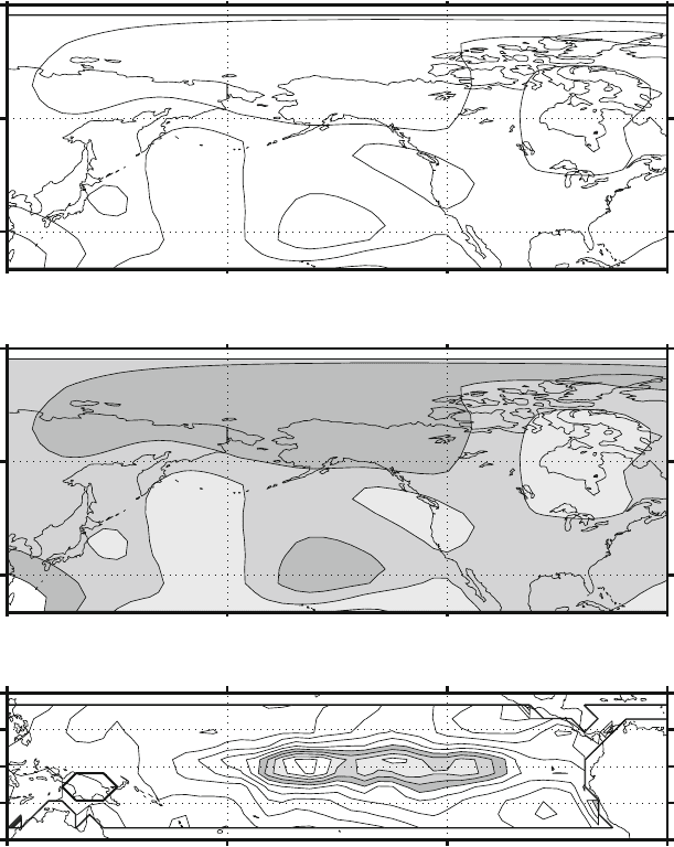
SST region to the South Atlantic, more precisely the region between 20S and 70S.

Variance of Forced manifold for Z 25 %

00 0.10.1

0.1

0.20.2

0.2

0.3

0.4

0.3

0.2

0.4

0.3

60W120W180W120E

30N

60N

90N

30N

60N

90N

Variance of Free manifold for Z 75 %

000.10.1 0.20.2 0.30.3 0.40.4 0.50.5

0.6

0.7

0.8

0.9

0.6

0.7

0.8

Variance of S

0.1

0.1 0.1

0.1

0.2

0.3

30W 0

70S

60S

50S

40S

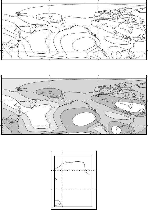
Fig. 8.2 Forced Manifold and Free Manifold. The picture represents the division in Forced and

Free Manifold for the North American geopotential ﬁeld Z in the region north of 20N and the

Atlantic SST in the region 20S–70S latitude. The top panel shows the ratio of the variance of the

Forced Manifold to the total variance, the middle panel shows the same for the Free Manifold.

The region used to examine the effect of the SST is in the bottom panel together with the total

variance of the SST. The amount of free variance is much larger than in the preceding case, showing

the minor impact of the Southern Atlantic SST on the geopotential in the North Paciﬁc

132 8 Multiple Linear Regression Methods

We have physical reasons to believe that the SST in this region are only modestly

connected with the activity over the North Paciﬁc. In fact the amount of variance

explained by the Forced manifold is much less than before and most of the variance

is in the Free Manifold, namely, mostly of the variance is not connected with the

variance of the SST in the South Atlantic.

The separation in (8.5) will allow us to study separately the properties of the

ﬁeld that is related to SST from what is independent. We are pretty free to choose

the forcing region and the study region any way we wish and so we can select them

on the basis of the various scientiﬁc hypotheses that we may think interesting. We

next see whether there are some basic properties that we can immediately point out.

The separation in Forced and Free manifold is not trivial, mostly because of the

non linear nature of the pseudoinverse used in the solution of the PRO method. We

have therefore no reasons to expect any particular relation between the structure of

the manifolds and the total ﬁeld. The variance structure is unrelated and we can

convince ourselves by examining the EOF of the total ﬁeld compared to those of the

two manifolds.

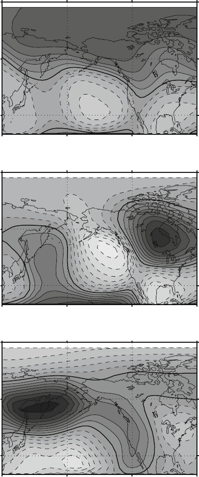
Figure 8.3 displays the ﬁrst three EOF modes of the geopotential over the

Paciﬁc/North American region. These show the familiar positive and negative

structures extending from the central tropical Paciﬁc ocean towards the American

continent. The following ﬁgure (Fig. 8.4) shows the same three modes but for the

Forced Manifold. The patterns are different. They show signiﬁcant increase in the

amplitude in the lower tropics ad other features that a more detailed analysis may

indicate. The last picture (Fig. 8.5) shows the same modes but for the Free Mani-

fold. This variability is unconnected with the tropical SST and we can see that the

amplitude is concentrated away from the tropics and in general the patterns are even

more different.

In this example we can use some of our meteorological expertise to interpret the

results and connect them to the phenomenon that they represent; in a particular ap-

plication one will have to do the same, by analyzing in detail the process to discuss

the modes in a scientiﬁcally meaningful way. It is clear however that the separa-

tion is real and that is not trivial, in the sense of simply selecting some particular

mode of variations over the others. The main reason for this behavior is the decrease

of degrees of freedom due to the pseudoinverse. The pseudoinverse eliminates the

degrees of freedom corresponding to zero singular values which are associated to

modes that do not contribute to be variance. Hence the Forced Manifold AS is not

the entire space Z. In the case of multiple realizations with the same S, the num-

ber of degrees of freedom of the data Z is not the number of realization times the

time levels, in our case 102, but only the smaller number of degrees of freedom

corresponding to the time levels for S, namely 34.

8.3 The Forced Manifold 133

−0.1−0.1 −0.05−0.05

120E 180W 120W 60W

30N

60N

90N

30N

60N

90N

30N

60N

90N

Total EOF Mode 1 33.4%

−0.1−0.1

−0.05

050.0−0

0.05

−0.05

0.05

Total EOF Mode 2 13.5%

−0.1−0.1 −0.05

−0.05

0.05

Total EOF Mode 3 9.4%

Fig. 8.3 EOF of the Total ﬁeld. The picture shows the ﬁrst three EOF modes for Z over the region

of the Paciﬁc/North America

134 8 Multiple Linear Regression Methods

−0.1−0.1 −0.05−0.05

−0.05

0.05

−0.05

120E 180W 120W 60W

30N

60N

90N

30N

60N

90N

30N

60N

90N

Forced EOF Mode 1 39.2%

−0.150.0−1.0−

−0.05

0.05

Forced EOF Mode 2 19.1%

−0.1−0.1

−0.05

Forced EOF Mode 3 9.3%

Fig. 8.4 As in Fig. 8.3, but for the Forced Manifold

8.3 The Forced Manifold 135

−0.1−0.1 −0.05−0.05

0.05

120E 180W 120W 60W

30N

60N

90N

120E 180W 120W 60W

30N

60N

90N

120E 180W 120W 60W

30N

60N

90N

Free EOF Mode 1 32.0%

−0.150.0−1.0−−0.05

0.05

−0.05

Free EOF Mode 2 13.4%

−0.150.0−1.0−−0.05

0.05

−0.05

Free EOF Mode 3 9.8%

Fig. 8.5 As in Fig. 8.3, but for the Free Manifold

136 8 Multiple Linear Regression Methods

8.3.1 Signiﬁcance Analysis

The PRO method can give us an easy way to ﬁnd connections between ﬁelds, how-

ever there is still the chance that some of the connections are just incidental. It would

be nice to have some method to estimate the probability that the separation is indeed

the result of casual relations.

To understand this point we need to go back to the operator A D ZS

.The

discussion is easier if we consider A under the scaling of Sect. 8.2.1. This choice is

no loss of validity with respect to the general case and the structure of A is simpler.

The deﬁnition of A means that the components of A are the time correlation between

the time series of the EOF of Z and S. The elements of A therefore can be written as

iD1

.i/s

.i/ a

iD1

.i/s

.i/ ::: a

iD1

.i/s

.i/

iD1

.i/s

.i/ a

iD1

.i/s

.i/ ::: a

iD1

.i/s

.i/

iD1

.i/s

.i/ a

iD1

.i/s

.i/ ::: a

iD1

.i/s

.i/

;

where N

and N

are the number of EOFs for Z and S that have been retained in the

analysis. The matrix is non-symmetric as the components a

and a

are in general

different. They are the correlation coefﬁcients of the time series of EOF mode 1 for

Z with EOF mode 2 for S and the correlation coefﬁcients for the time series of EOF

mode 2 of Z with EOF mode 1 of S. In fact they are indeed regression coefﬁcients

in the general case that in this scaling reduce to correlation coefﬁcients. We can see

then the matrix A expresses the inﬂuence of each mode of one ﬁeld on the modes of

the other ﬁeld as in the following scheme

S.1/ ! Z.1/ S.1/ ! Z.2/ ::: S.1/ ! Z.N

S.2/ ! Z.1/ S.2/ ! Z.2/ ::: S.2/ ! Z.N

S.N

/ ! Z.1/ S.N

/ ! Z.2/::: S.N

/ ! Z.N

; (8.9)

or introducing the numerical values for the elements

8.3 The Forced Manifold 137

0:4023 0:0126 0:2145 0:0758 : : :

0:5741 0:2645 0:0249 0:0797 : : :

0:0491 0:0129 0:0787 0:1200 : : :

0:1705 0:4186 0:0880 0:1497 : : :

0:2999 0:1294 0:2053 0:0469 : : :

; (8.10)

where we have shown the ﬁrst few rows and columns of A. We can see that we can

use A to inspect the strength and the characteristic of the correlation an/or regres-

sion between each particular modes and the others. The arguments is not limited

by the choice of the representation in EOF. If we had elected to used the grid point

or station representation, the operator A could have been interpreted in the same

way. In that case the elements a

would have contained the correlation/regression

coefﬁcient for grid point i of Z with grid point or station j of S.

The description in (8.10)and(8.9) indicates that we have a statistical interpreta-

tion for A. Such an interpretation may be used to establish conﬁdence limits in the

numerical vales of the components of A. We can used heuristic methods to estab-

lish the baseline values that we can attribute to chance. For instance, in the previous

sections we have changed the analysis domain to regions where we were expecting

varying strengths of the relationship between S and Z. We can have an idea of the

sensitivity of the analysis by also scrambling in time one of the ﬁelds and using

the method to estimate the possibility of casual relations. The results are shown in

Fig. 8.6.

Here we can see that the amount of variance in the Forced Manifold has de-

creased by a large amount. This level is basically equivalent to the determination of

a zero level, that is the value that is generated by casual relations in the data. The

amount of Forced variance found is very close to the level determined by the exam-

ple in Fig. 8.2 where we used a physically based argument to estimate the level of

no relation, form the result of the scrambled test we can be rather conﬁdent that the

relation found in Fig. 8.1 is relatively robust.

We can have a more rigorous estimation of conﬁdence if we recognize that

the correlation/regression coefﬁcients in A can be tested against a Student’s

t-distribution. The test estimates the probability that the true coefﬁcient is in-

deed zero. The acceptable values for the probability levels in order to accept the

computed values is, of course, matter of choice, but usually values of 5%or1%are

used. These choices correspond to the statement that there a 5%or1% probability

that the hypothesis that the true value is indeed zero is true. We can insert this pro-

cess into the calculation of the Forced Manifold by testing each element of A and

putting to zero those components that pass the test. We can repeat the calculation

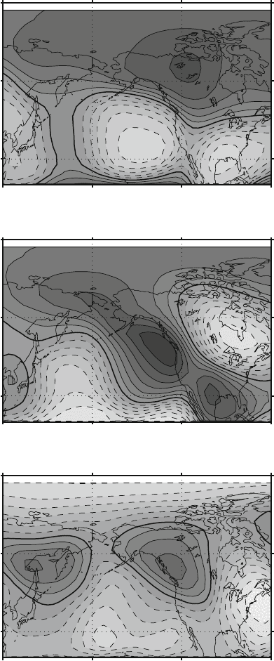
for Fig. 8.1 introducing now the signiﬁcance test at 1%. The results are shown in

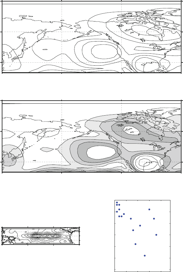
Fig. 8.7.

The Forced and Free manifolds for the geopotential and the tropical SST have

a similar distribution as in Fig. 8.7. Overall the total amount of variance that can

be attributed with conﬁdence to the forcing S is decreased, but the distribution has

concentrated and the difference between maxima and minima has increased. The

138 8 Multiple Linear Regression Methods

Scrambled case − Variance of Forced Manifold for Z 26 %

00 0.10.1 0.2

0.2

0.3

0.2

0.3

0.2

0.3

0.4

0.2

60W120W180W120E

30N

60N

90N

Variance of Free Manifold for Z 74 %

00 0.10.1 0.20.2 0.30.3 0.40.4 0.50.5 0.60.6

0.7

0.8

0.7

0.8

0.9

30N

60N

90N

Variance of S

0.1

0.2

0.3

0.4

0.5

0.6

0.7

0.1

0.8

0.1

0.9

0.1

0.2

0.1

0.5

0.9

0.2

20S

10S

10N

20N

Fig. 8.6 As in Fig. 8.1, but for a randomly permuted ﬁeld in time. The amount of variance that such

casual relations detect is much lower than in the original picture, giving us some conﬁdence in the

determination of the original A. The amount of variance found is also very close to the physically

motivated examples of Fig. 8.2, adding more conﬁdence to the robustness of the original estimation

coefﬁcients of the operator A that are signiﬁcant according to the Student t-test

are indicated in the top right panel and they have been retained in the calculation,

whereas the other have been put to zero. The signiﬁcance test makes it easy to deal

with the time scrambled case (Fig. 8.8). There is no coherent pattern in the Z ﬁeld

and the relations seem completely casual.

8.3 The Forced Manifold 139

0 5 10 15 20

nz = 16

A − Significance tested for 1%

Variance of Forced manifold for Z 16 %

0.1

0.2

0.3

0.1

0.4

0.2

60W120W180W120E

30N

60N

90N

30N

60N

90N

Variance of Free manifold for Z 84 %

000.10.1 0.20.2 0.30.3 0.40.4 0.50.5 0.60.60.6 0.7

0.7

0.8

0.80.8

0.9

0.7

0.6

0.8

0.5

0.9

0.6

0.4

0.8

0.9

Variance of S

0.1

0.2

0.3

0.4

0.5

0.6

0.7

0.1

0.8

0.1

0.9

0.1

120E 180W 120W 60W

20S

10S

10N

20N

Fig. 8.7 Forced and Free manifolds for the tropical SST, as in Fig. 8.7 but including a signiﬁcance

test. The coefﬁcients of the operator A that are signiﬁcant according to the t-Student test are indi-

cated in the top right panel and they have been retained in the calculation. The left panels show

the Forced and Free Manifolds variance: although overall the total amount of variance that can

be attributed with conﬁdence to the forcing S is decreased, the distribution has peaked and it has

intensiﬁed