Navarra Antonio, Simoncini Valeria. A Guide to Empirical Orthogonal Functions for Climate Data Analysis

Подождите немного. Документ загружается.

5.3 Complex EOF 79

The oblique patterns are then given by

promax

D VTD;

where the matrix D scales the oblique modes to unit length, namely

D diag.T



1

The deﬁnition of the target matrix as a power of the original pattern (cf. the exponent

k in (5.5)) is an attempt to emphasize the differences between maxima and minima,

to obtain a simpler structure in which intermediate values are unfavored. The value

of the parameter k is arbitrary, but there is a difference in the sensitivity of the

modes according to the shape of the sought after real pattern. If we expect a strong

pattern with large variations between its extreme values, then k should be set to a

low number. In practice, k D 2 or k D 4 are often used.

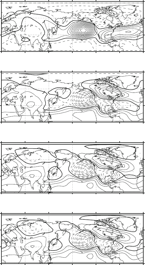
The comparison between the standard and rotated modes is shown in Fig. 5.4

for the ﬁrst mode in the test data set for Z500. The orthogonal VARIMAX rota-

tion results in an intense pattern, better localized, as we have seen in the preceding

pictures. The PROMAX solution (lower panels) obtains patterns even more local-

ized on North America, but we can notice one of the problems with PROMAX,

especially if a large value of k is selected (bottom panel is for k D 12). The con-

struction of these modes tends to polarize the spatial variability, concentrating the

variance in smaller regions. The modes have fewer peaks, but of larger amplitude.

We can see that for k D 12 the centers are more intense, even in regions where the

EOF or the VARIMAX showed little amplitude. This example emphasizes that sim-

ple structure in principle that does not necessarily imply more meaningful modes.

Figure 5.1 shows that from the point of view of simple structure, i.e. the polariza-

tion and separation of the pattern values in space, we are getting better every time.

The concept of simple structure is therefore a very useful concept, but it cannot be

considered as the only guiding principle.

Oblique modes have not found a widespread usage in data analysis, perhaps be-

cause of the parametric freedom, but also because they cannot be used to separate

the variance.

5.3 Complex EOF

We have seen how conventional and rotated EOF can be employed to identify pat-

terns that optimize the explanation of the variance. EOF identify the dominant

pattern, but the information on the time evolution is only implicitly included into

the evolution of the coefﬁcients. Data that contain oscillations in time or in space

and time as a propagating signal, are very common in applications. In Sect. 4.5.1

we have seen an example in which the standard EOF have been applied to an ideal

example of a propagating wave. The signature of the propagation is visible in the

80 5 Generalizations: Rotated, Complex, Extended and Combined EOF

EOF

-0.2-0.2 -0.15-0.15 -0.1-0.1 -0.05-0.05

0.05

0.1

VARIMAX

-0.2-0.2 -0.15-0.15 -0.1-0.1 -0.05-0.05

-0.05

-0.1

PROMAX K=2

-0.2-0.2 -0.15-0.15 -0.1-0.1 -0.05-0.05

-0.05

PROMAX K=12

-0.2-0.2 -0.15-0.15 -0.1-0.1 -0.05-0.05

-0.05

0°

60°W120°W

120°E

60°E

180°W

0°

60°W120°W

120° E

60° E

180°W

0°

60°W120°W

120° E

60° E

180°W

0°

60°W120°W

120° E

60° E

180°W

0°

60°W120°W

120° E

60° E

180°W

0°

60°N

30°N

90°N

0°

60°N

30°N

90°N

0°

60°N

30°N

90°N

0°

60°N

30°N

90°N

0°

Fig. 5.4 Conventional, rotated and PROMAX (oblique) EOF for the test data sets Z500

5.3 Complex EOF 81

EOF, but it requires some indirect interpretation. The presence of propagation is in-

dicated by two modes whose patterns are in quadrature, namely the relative maxima

and minima of one pattern correspond to the zero lines of the other and the two EOF

explain a similar amount of variance (see Fig. 4.13).

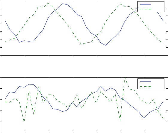
The variations of the coefﬁcients in time (top panel of Fig. 5.5) show a periodic

behavior in time. There is a shift in time corresponding to a quarter of a wavelength

between EOF1 and EOF2. A quarter wavelength shift in time is the phase lag typical

of a harmonic wave of the form

V.x;t/ D<ŒU.x/e

i!t

 D<ŒU.x/.cos.!t/ C { sin.!t//: (5.6)

Therefore, the variation in time of the EOF coefﬁcient seems to identify a kind

of variability that can be expressed as a harmonic wave with real part EOF1 and

imaginary part EOF2. The EOF analysis has been able to ﬁnd couples of modes that

are strongly linked, in fact they may be part of the same physical system.

Waves are a pervasive physical phenomenon so it is not surprising that the EOF’s

feature of detecting propagating modes has raised considerable interest. On the other

hand, it is also true that this capability is a sort of byproduct of the general property

of EOF to maximize variance. Would it be possible to sharpen the EOF deﬁnition

so as to go after propagating modes?

0 5 10 15 20 25 30 35

−0.4

−0.3

−0.2

−0.1

0.1

0.2

0.3

Time coefficients for propagating wave

EOF 1

EOF 2

0 5 10 15 20 25 30 35

−0.6

−0.4

−0.2

0.2

0.4

Time coefficients for stationary wave

EOF 1

EOF 2

Fig. 5.5 EOF coefﬁcients of the example in Sect. 4.5. Top panel: a propagating wave. Bottom

panel: a stationary wave

82 5 Generalizations: Rotated, Complex, Extended and Combined EOF

We have seen that the quarter wavelength shift is a peculiar phase relation that

indicates propagation. Can we ﬁnd a way to enhance the modes that are in that

particular phase relation? One possibility is to change the available data to stress

the phase relation we are looking for; in our case we can expand the data by adding

a new data set obtained by shifting all data by one quarter wavelength. This is a

mathematical procedure that can be performed by Hilbert transform. The analytical

deﬁnition of the transform is

f D HŒf.x;t/ D



1

s./

t  

d

where the integral is to be understood to be a Cauchy principal value to avoid the

singularities at inﬁnity and at t D . In practice, the transform of discrete signal is

performed using a discrete Fourier transform (Hahn 1996)

f D HŒf.x;t/ D

.x; !/e

2{!t

.x; !/ D

ig.x;!/ for !>0

0 for ! D 0

ig.x;!/ for !<0:

where g.!/ is the discrete Fourier transform of f . The Hilbert transform shifts the

data series a quarter period to obtain a new, augmented, data series of complex data,

D X C iH.X/;

where the real part contains the original data and the imaginary data the quarter

period shifted data. Let us assume that X

has been detrended, so that its mean is

zero. The variance is thus given by the sum of the diagonal elements of the following

matrix



D XX



C H.X/



H.X/ C i.X.H.X//



 H.X/X



/: (5.7)

Therefore, the variance of the new data set X

is twice the variance of the origi-

nal data series, as the imaginary term does not contribute to the variance. However,

the balance in the imaginary term is rather delicate and it often happens that in real

cases affected by noise, the variance is only approximately twice the original vari-

ance of the data. Complex EOF deﬁned through Hilbert transforms will therefore

try to optimize variance using patterns that are complex and whose real and imagi-

nary parts are shifted by a quarter period. Below is a Matlab implementation of this

procedure, that was used to generate later plots.

function [u,lam,v,proj]=ceof(z,indf,nmode,nproj)

% Compute complex EOF of z and expand it for nmode modes

% Inputs:

% z Data Matrix

% indf Index for the data

5.3 Complex EOF 83

% nmode Number of EOF to return

% nproj Number of EOF to generate projections

% Outputs:

% u EOF arrays (nspace x nmode)

% lam variance explained (ntime)

% v Unnormalized EOF coefficients

% proj Projection on the nmode EOF

resol = [96 48];

zh=hilbert(z);

[uu,ss,v]=svd(zh,0);

lam = diag(ss).ˆ2/sum(diag(ss).ˆ2); % Explained variances

u=zeros([resol(1)

resol(2) nmode]); % Keep Only first modes

u(indf,1:nmode)=uu(indf,1:nmode);

proj=zh’

uu(:,1:nproj); % Compute projections

return

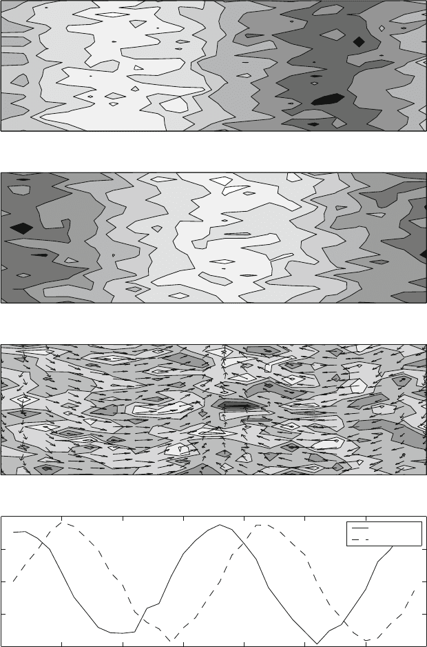
Figure 5.6 shows the ﬁrst complex EOF (CEOF 1) for the case of the analytical

wave of Sect. 4.5.1. The top panels show the real and imaginary parts of the ﬁrst

mode and they display the familiar shape in quadrature one with the other. The real

and imaginary parts of the coefﬁcient are also shifted one quarter wavelength. We

can see that the CEOF has recovered the propagating wave hidden in the noise.

Being focused on extracting the signals that are shifted one quarter wavelength,

the CEOF are very efﬁcient at doing that, but at the same time the Complex EOF

do not comparably perform if the oscillatory signal has a structure with a different

phase relation. For instance, if the signal is stationary, namely it changes in time

without a change of phase in space, like an oscillating beam, CEOF run into trouble.

Propagation and stationarity are identiﬁed clearly in our ideal experiment by simple

EOF (Fig. 5.5) because the stationary signal (bottom panel) shows no clear phase

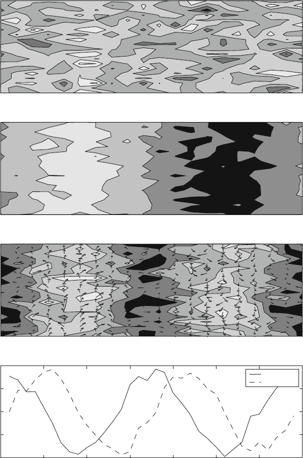
relation between the time series of the coefﬁcient. Application of the CEOF to a

stationary signal (Fig. 5.7) produces a spatial pattern that bears indication of the

signal stationary nature. Only the real or imaginary component is now needed to

give the spatial structure of a stationary signal, in this case the real part, whereas the

other component is usually noise, without a clear pattern. It would appear that CEOF

have successfully identiﬁed the signal, however if one looks at the time coefﬁcient

(bottom panel) it is possible to see that both time coefﬁcients oscillate, pretty much

in the same way as in the preceding propagating case. CEOF can only distinguish

between spatial propagation and lack of it, implying the absence of spatial phase

relations; in general, however, the inspection of the time coefﬁcient alone is not

sufﬁcient to distinguish between them. As an example, in Fig. 5.6 it is possible

to see that the variation of the spatial phase (the arrows in the panel) is organized

and smooth, corresponding to the organized propagation. In contrast, in Fig. 5.7

the phase variation is disorganized and dominated by noise. This investigation can

be somewhat difﬁcult to perform with real data, where spatial phase relations are

84 5 Generalizations: Rotated, Complex, Extended and Combined EOF

2 4 6 8 10 12 14 16 18 20

Real Part CEOF 1 37%

2 4 6 8 10 12 14 16 18 20

Imaginary Part CEOF 1 37%

2 4 6 8 10 12 14 16 18 20

Phase and Amplitude CEOF 1 37%

0 5 10 15 20 25 30 35

–0.2

–0.1

0.1

0.2

Time coefficients for propagating wave

Real Part

Imag Part

Fig. 5.6 First complex EOF of the analytical example. Top panels: spatial patterns of the real and

imaginary parts, then the amplitude and phases of the mode. In the title, the explained variance is

recorded. Bottom panel: time evolution of the coefﬁcient

5.3 Complex EOF 85

2 4 6 8 10 12 14 16 18 20

Real Part CEOF 1 23%

2 4 6 8 10 12 14 16 18 20

Imaginary Part CEOF 1 23%

2 4 6 8 10 12 14 16 18 20

Phase and Amplitude CEOF 1 23%

0 5 10 15 20 25 30 35

–0.2

–0.1

0.1

0.2

Time coefficients

Real Part

Imag Part

Fig. 5.7 As in Fig. 5.6 but for the case of a stationary wave

86 5 Generalizations: Rotated, Complex, Extended and Combined EOF

difﬁcult to identify. In practice Complex EOF cannot be used to distinguish between

propagating and non-propagating (i.e. stationary) oscillations.

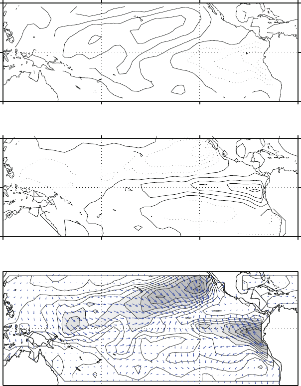
A complex analysis of the test data set for SST yields the result shown in Fig. 5.8.

This picture displays the second mode represented in its real and imaginary compo-

nents. The top panel is the real part, showing a mode of variability concentrated in

the equatorial area, the middle panel is the imaginary component of the mode. The

0.02

CEOF 2 −− Real Part

−0.06

−0.02

CEOF 2 −− Imaginary Part

CEOF 2 −− Amplitude and Phase

30°N

30°S

120°E 60°W

180°W

120°W

120°E 60°W

180°W

120°W

120E

60W

180E

120W

0°

30°N

30°S

0°

30N

30S

Fig. 5.8 Second complex EOF of the marine temperatures in the Paciﬁc. Top panel: real compo-

nent, middle panel: imaginary component, lower panel: amplitude and phase

5.4 Extended EOF 87

1960 1965 1970 1975 1980 1985 1990 1995

0.05

0.1

0.15

0.2

Amplitude of CEOF 1

1965 1970 1975 1980 1985 1990 1995

Temporal Phase of CEOF 1

Phase angle (2π)

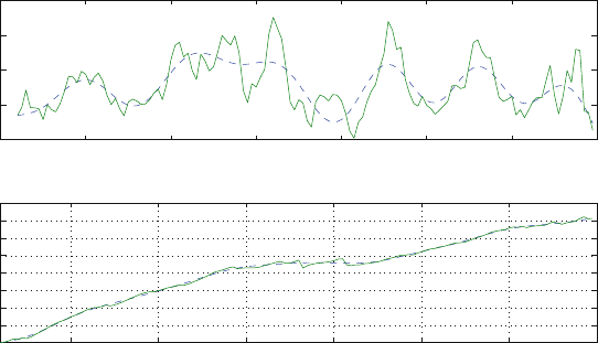
Fig. 5.9 Time series of the coefﬁcient of the second Complex EOF shown in the previous picture.

The top panel shows the amplitude of the complex coefﬁcient, whereas the bottom panel shows

the evolution of the unwrapped phase angle. The phase velocity is obtained as the derivative of the

phase, showing an acceleration after 1980

bottom panel is the representation in amplitude and phase. The amplitude is con-

centrated in the east equatorial Paciﬁc, the rotation of the phase indicates a phase

velocity towards the west. Here the convention used is that the phase arrows point

to the east if the real part is positive and the imaginary part is zero.

The time evolution of the mode coefﬁcient is displayed in Fig. 5.9, indicating the

periods of time in which such a mode is more or less energetic. The “unwrapped”

phase, that is the phase of the time coefﬁcient reduced to a single-value function by

adding a factor 2 every time it crosses the zero line, also shows different phase

speed from a period to the next.

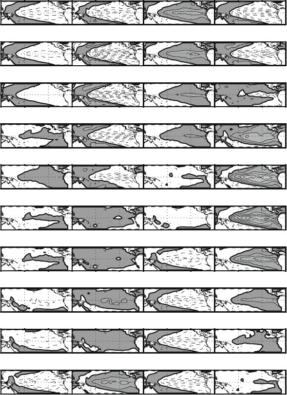
Figure 5.10 shows the modal actual evolution, cycling through the real and imagi-

nary parts with alternate signs. The reported ﬁeld is only based on the reconstruction

of the second mode, starting from 1980 onward. The picture shows that the CEOF

indicates an oscillatory behavior that can also be aperiodic in time. There are pe-

riods in which oscillations are clearly visible, and periods where oscillations are

quiescent and there is very little appearance of the mode. This is a good example of

the capability of the CEOF to capture irregular oscillations.

5.4 Extended EOF

Complex EOF are based on the analysis of variance by taking into account the data

time behavior. This is done by creating a new data set that includes the original data

series and a new series that is shifted by a quarter wavelength. The Hilbert transform

88 5 Generalizations: Rotated, Complex, Extended and Combined EOF

COMPLEX EOF

51%

Fig. 5.10 Time evolution of the second for SST from Winter 1980 (top left panel) for each con-

secutive season. Time is increasing downwards and from left to right. The 1982–1983 El Ni˜no

event is visible in the ﬁrst and second column on the left

makes the procedure very rigorous. However, it is sometimes desirable to use a less

rigorous approach and to gain some ﬂexibility in the process. Complex EOF change

the state vectors in a way that the basic data are not the data at a given time, but the

combination data at a single time plus data shifted one quarter wavelength in time.

A possible alternative is to introduce a derivative EOF analysis that crudely realizes