Neamen D. Microelectronics: Circuit Analysis and Design

Подождите немного. Документ загружается.

18 Part 1 Semiconductor Devices and Basic Applications

where

is a constant called the hole mobility, and again has units of cm

/V–s.

For low-doped silicon, the value of

is typically 480 cm

/V–s, which is less

than half the value of the electron mobility. The positive sign in Equation (1.9) in-

dicates that the hole drift velocity is in the same direction as the applied electric

field as shown in Figure 1.8(b). The hole drift produces a drift current density J

(A/cm

) given by

=+epv

=+ep(+μ

E) =+epμ

(1.10)

where p is the hole concentration (#/cm

) and e is again the magnitude of the elec-

tronic charge. The conventional drift current is in the same direction as the ﬂow of

positive charge, which means that the drift current in a p-type material is also in the

same direction as the applied electric ﬁeld.

Since a semiconductor contains both electrons and holes, the total drift current

density is the sum of the electron and hole components. The total drift current den-

sity is then written as

J = enμ

E +epμ

E = σ E =

(1.11(a))

where

σ = enμ

+epμ

(1.11(b))

and where

is the conductivity of the semiconductor in

(

–cm)

−1

and where

ρ = 1/σ

is the resistivity of the semiconductor in

(

–cm). The conductivity is re-

lated to the concentration of electrons and holes. If the electric ﬁeld is the result of

applying a voltage to the semiconductor, then Equation (1.11(a)) becomes a linear

relationship between current and voltage and is one form of Ohm’s law.

From Equation (1.11(b)), we see that the conductivity can be changed from

strongly n-type,

n  p

, by donor impurity doping to strongly p-type,

p  n

,by

acceptor impurity doping. Being able to control the conductivity of a semicon-

ductor by selective doping is what enables us to fabricate the variety of elec-

tronic devices that are available.

EXAMPLE 1.3

Objective: Calculate the drift current density for a given semiconductor.

Consider silicon at

T = 300 K

doped with arsenic atoms at a concentration

= 8 ×10

−3

. Assume mobility values of

= 1350

/V–s and

480 cm

/V–s. Assume the applied electric ﬁeld is 100 V/cm.

Solution: The electron and hole concentrations are

∼

= 8 ×10

−3

and

p =

(1.5 × 10

)

8 × 10

= 2.81 ×10

−3

Because of the difference in magnitudes between the two concentrations, the con-

ductivity is given by

σ = eμ

n + eμ

∼

eμ

nea80644_ch01_07-066.qxd 06/08/2009 05:15 PM Page 18 F506 Tempwork:Dont' Del Rakesh:June:Rakesh 06-08-09:MHDQ134-01 Folder:MHDQ134-01:

Chapter 1 Semiconductor Materials and Diodes 19

σ = (1.6 × 10

−19

)(1350)(8 × 10

) = 1.73(–cm)

−1

The drift current density is then

J = σ E = (1.73)(100) = 173 A/cm

Comment: Since

n  p

, the conductivity is essentially a function of the electron

concentration and mobility only. We may note that a current density of a few hundred

amperes per square centimeter can be generated in a semiconductor.

EXERCISE PROBLEM

Ex 1.3: Consider n-type GaAs at

T = 300 K

doped to a concentration of

= 2 ×10

−3

. Assume mobility values of

= 6800

/V–s and

300 cm

/V–s. (a) Determine the resistivity of the material. (b) Determine the ap-

plied electric ﬁeld that will induce a drift current density of 175 A/cm

. (Ans.

(a)

0.0460 –cm

, (b) 8.04 V/cm).

Note: Two factors need to be mentioned concerning drift velocity and mobility.

Equations (1.7) and (1.9) imply that the carrier drift velocities are linear functions of

the applied electric ﬁeld. This is true for relatively small electric ﬁelds. As the elec-

tric ﬁeld increases, the carrier drift velocities will reach a maximum value of ap-

proximately 10

cm/s. Any further increase in electric ﬁeld will not produce an

increase in drift velocity. This phenomenon is called drift velocity saturation.

Electron and hole mobility values were given in Example 1.3. The mobility val-

ues are actually functions of donor and/or acceptor impurity concentrations. As the

impurity concentration increases, the mobility values will decrease. This effect then

means that the conductivity, Equation (1.11(b)), is not a linear function of impurity

doping.

These two factors are important in the design of semiconductor devices, but will

not be considered in detail in this text.

Diffusion Current Density

In the diffusion process, particles ﬂow from a region of high concentration to a region

of lower concentration. This is a statistical phenomenon related to kinetic theory. To

explain, the electrons and holes in a semiconductor are in continuous motion, with an

average speed determined by the temperature, and with the directions randomized by

interactions with the lattice atoms. Statistically, we can assume that, at any particular

instant, approximately half of the particles in the high-concentration region are

moving away from that region toward the lower-concentration region. We can also

assume that, at the same time, approximately half of the particles in the lower-

concentration region are moving toward the high-concentration region. However, by

deﬁnition, there are fewer particles in the lower-concentration region than there are in

the high-concentration region. Therefore, the net result is a ﬂow of particles away

from the high-concentration region and toward the lower-concentration region. This

is the basic diffusion process.

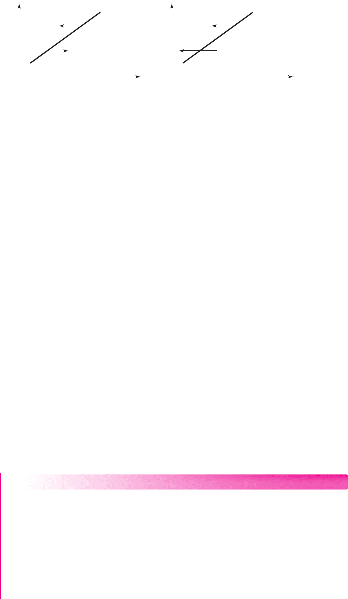
For example, consider an electron concentration that varies as a function of distance

x, as shown in Figure 1.9(a). The diffusion of electrons from a high-concentration region

nea80644_ch01_07-066.qxd 06/08/2009 05:15 PM Page 19 F506 Tempwork:Dont' Del Rakesh:June:Rakesh 06-08-09:MHDQ134-01 Folder:MHDQ134-01:

20 Part 1 Semiconductor Devices and Basic Applications

to a low-concentration region produces a ﬂow of electrons in the negative x direction.

Since electrons are negatively charged, the conventional current direction is in the

positive x direction.

The diffusion current density due to the diffusion of electrons can be written as

(for one dimension)

= eD

(1.12)

where e, in this context, is the magnitude of the electronic charge, dn/dx is the gra-

dient of the electron concentration, and D

is the electron diffusion coefﬁcient.

In Figure 1.9(b), the hole concentration is a function of distance. The diffusion

of holes from a high-concentration region to a low-concentration region produces a

ﬂow of holes in the negative x direction. (Conventional current is in the direction of

the ﬂow of positive charge.)

The diffusion current density due to the diffusion of holes can be written as (for

one dimension)

=−eD

(1.13)

where e is still the magnitude of the electronic charge, dp/dx is the gradient of the

hole concentration, and D

is the hole diffusion coefﬁcient. Note the change in sign

between the two diffusion current equations. This change in sign is due to the differ-

ence in sign of the electronic charge between the negatively charged electron and the

positively charged hole.

EXAMPLE 1.4

Objective: Calculate the diffusion current density for a given semiconductor.

Consider silicon at

T = 300 K

. Assume the electron concentration varies lin-

early from

n = 10

−3

n = 10

−3

over the distance from

x = 0

x = 3 μ

m. Assume

= 35

/s.

Solution: We have

= eD

n

x

= (1.6 ×10

−19

)(35)



−10

0 − 3 ×10

−4



Electron

diffusion

Electron diffusion

current density

Hole

diffusion

Hole diffusion

current density

(a) (b)

Figure 1.9 (a) Assumed electron concentration versus distance in a semiconductor, and

the resulting electron diffusion and electron diffusion current density, (b) assumed hole

concentration versus distance in a semiconductor, and the resulting hole diffusion and hole

diffusion current density

nea80644_ch01_07-066.qxd 06/08/2009 05:15 PM Page 20 F506 Tempwork:Dont' Del Rakesh:June:Rakesh 06-08-09:MHDQ134-01 Folder:MHDQ134-01:

Chapter 1 Semiconductor Materials and Diodes 21

= 187 A/cm

Comment: Diffusion current densities on the order of a few hundred amperes per

square centimeter can also be generated in a semiconductor.

EXERCISE PROBLEM

Ex 1.4: Consider silicon at

T = 300 K

. Assume the hole concentration is given

p = 10

−x/L

(cm

−3

), where

= 10

−3

. Calculate the hole diffusion

current density at (a)

x = 0

and (b)

x = 10

−3

. Assume

= 10

/s. (Ans.

(a) 16 A/cm

, (b) 5.89 A/cm

)

The mobility values in the drift current equations and the diffusion coefﬁcient

values in the diffusion current equations are not independent quantities. They are

related by the Einstein relation, which is

∼

0.026 V

(1.14)

at room temperature.

The total current density is the sum of the drift and diffusion components. For-

tunately, in most cases only one component dominates the current at any one time in

a given region of a semiconductor.

DESIGN POINTER

In the previous two examples, current densities on the order of 200 A/cm

have

been calculated. This implies that if a current of 1 mA, for example, is required in

a semiconductor device, the size of the device is small. The total current is given

I = JA

, where A is the cross-sectional area. For

I = 1mA= 1 ×10

−3

A and

J = 200

A/cm

, the cross-sectional area is

A = 5 ×10

−6

. This simple calcu-

lation again shows why semiconductor devices are small in size.

Excess Carriers

Up to this point, we have assumed that the semiconductor is in thermal equilibrium.

In the discussion of drift and diffusion currents, we implicitly assumed that equilib-

rium was not signiﬁcantly disturbed. Yet, when a voltage is applied to, or a current

exists in, a semiconductor device, the semiconductor is really not in equilibrium.

In this section, we will discuss the behavior of nonequilibrium electron and hole

concentrations.

Valence electrons may acquire sufﬁcient energy to break the covalent bond and

become free electrons if they interact with high-energy photons incident on the semi-

conductor. When this occurs, both an electron and a hole are produced, thus generating

1.1.4

nea80644_ch01_07-066.qxd 06/08/2009 05:15 PM Page 21 F506 Tempwork:Dont' Del Rakesh:June:Rakesh 06-08-09:MHDQ134-01 Folder:MHDQ134-01:

22 Part 1 Semiconductor Devices and Basic Applications

an electron–hole pair. These additional electrons and holes are called excess

electrons and excess holes.

When these excess electrons and holes are created, the concentrations of free

electrons and holes increase above their thermal equilibrium values. This may be rep-

resented by

n = n

+δn

(1.15(a))

and

p = p

+δp

(1.15(b))

where

and

are the thermal equilibrium concentrations of electrons and holes,

and

n and

p are the excess electron and hole concentrations.

If the semiconductor is in a steady-state condition, the creation of excess

electrons and holes will not cause the carrier concentration to increase indefi-

nitely, because a free electron may recombine with a hole, in a process called

electron–hole recombination. Both the free electron and the hole disappear

causing the excess concentration to reach a steady-state value. The mean time

over which an excess electron and hole exist before recombination is called the

excess carrier lifetime.

Excess carriers are involved in the current mechanisms of, for example, solar

cells and photodiodes. These devices are discussed in Section 1.5.

Test Your Understanding

TYU 1.1 Determine the intrinsic carrier concentration in silicon, germanium, and

GaAs at (a)

T = 400 K

and (b)

T = 250 K

. (Ans. (a) Si:

= 4.76 ×10

−3

Ge:

= 9.06 ×10

−3

, GaAs:

= 2.44 ×10

−3

; (b) Si:

= 1.61 ×

−3

, Ge:

= 1.42 ×10

−3

, GaAs:

= 6.02 ×10

−3

)

TYU 1.2 (a) Consider silicon at

T = 300 K

. Assume that

= 1350

/V–s

and

= 480 cm

/V–s

. Determine the conductivity and resistivity if (a)

= 2 ×10

−3

and (b)

= 2 ×10

−3

. (Ans. (a)

σ = 0.154 (–cm)

−1

ρ = 6.51 –cm

; (b)

σ = 43.2 (–cm)

−1

,ρ= 0.0231 –cm).

TYU 1.3 Using the results of TYU1.2, determine the drift current density if an

electric ﬁeld of 4 V/cm is applied to the semiconductor. (Ans. (a) 0.616 A/cm

(b) 172.8 A/cm

TYU 1.4 The electron and hole diffusion coefﬁcients in silicon are

= 35

and

= 12.5

/s, respectively. Calculate the electron and hole diffusion current

densities (a) if an electron concentration varies linearly from

n = 10

−3

n = 10

−3

over the distance from

x = 0

x = 2.5 μ

m and (b) if a hole con-

centration varies linearly from

p = 10

−3

p = 5 ×10

−3

over the dis-

tance from

x = 0

x = 4.0 μ

m. (Ans. (a)

= 202

A/cm

, (b)

=−24.5

A/cm

)

TYU 1.5 A sample of silicon at

T = 300 K

is doped to

= 8 ×10

−3

. (a) Cal-

culate

and

. (b) If excess holes and electrons are generated such that their

respective concentrations are

δn = δp = 10

−3

, determine the total concentra-

tions of holes and electrons. (Ans. (a)

= 8 ×10

−3

= 2.81 ×10

−3

;

(b)

n = 8.1 × 10

−3

p ≈ 10

−3

)

nea80644_ch01_07-066.qxd 06/08/2009 05:15 PM Page 22 F506 Tempwork:Dont' Del Rakesh:June:Rakesh 06-08-09:MHDQ134-01 Folder:MHDQ134-01:

Chapter 1 Semiconductor Materials and Diodes 23

(a) (c)

x = 0

Doping

concentration

(b)

x = 0

Cross-sectional

area

x = 0

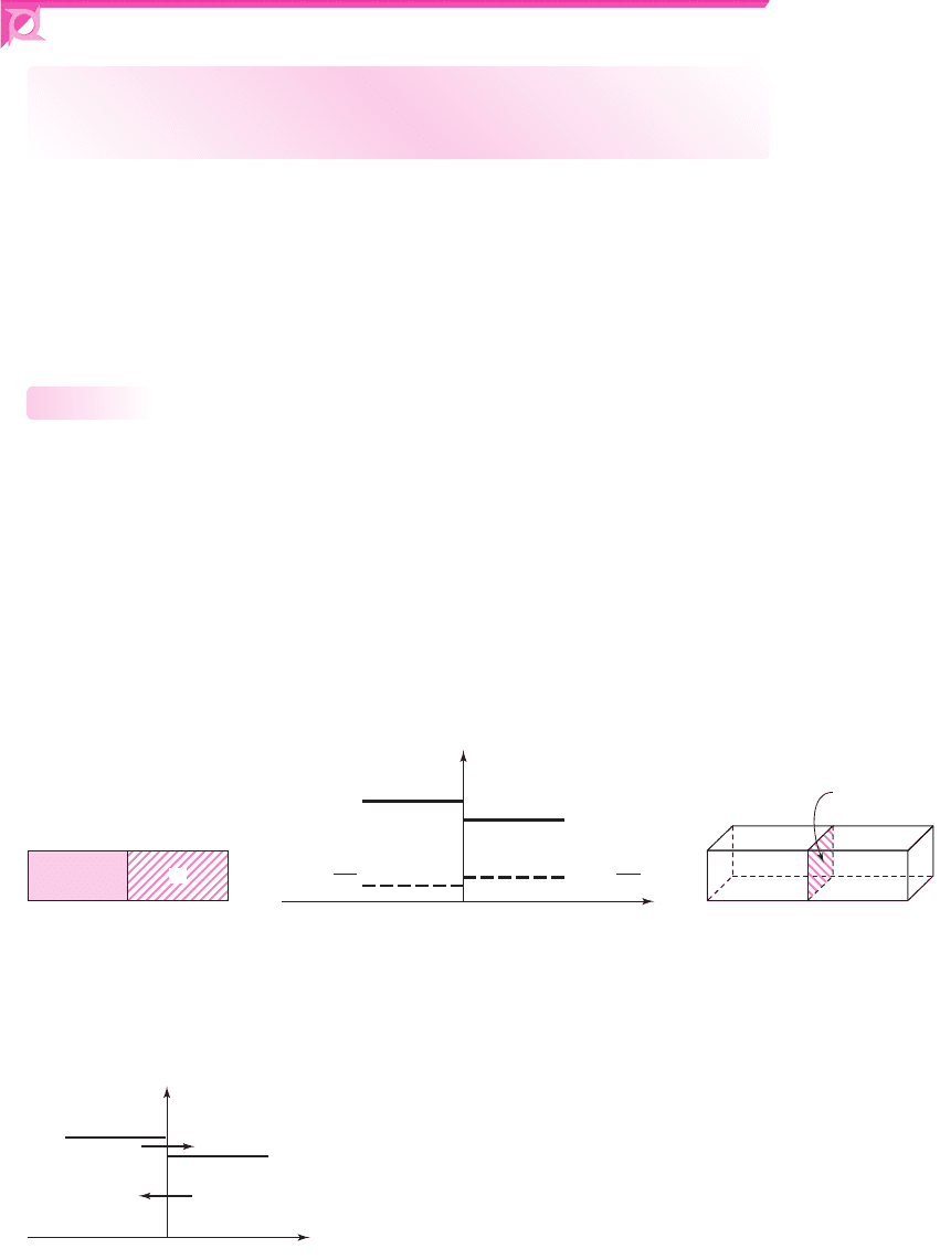
Figure 1.10 (a) The pn junction: (a) simpliﬁed one-dimensional geometry, (b) doping proﬁle

of an ideal uniformly doped pn junction, and (c) three-dimensional representation showing

the cross-sectional area

1.2 THE pn JUNCTION

Objective: • Determine the properties of a pn junction including the

ideal current-voltage characteristics of the pn junction diode.

In the preceding sections, we looked at characteristics of semiconductor materials.

The real power of semiconductor electronics occurs when p- and n-regions are di-

rectly adjacent to each other, forming a pn junction. One important concept to

remember is that in most integrated circuit applications, the entire semiconductor

material is a single crystal, with one region doped to be p-type and the adjacent

region doped to be n-type.

The Equilibrium pn Junction

Figure 1.10(a) is a simpliﬁed block diagram of a pn junction. Figure 1.10(b) shows

the respective p-type and n-type doping concentrations, assuming uniform doping in

each region, as well as the minority carrier concentrations in each region, assuming

thermal equilibrium. Figure 1.10(c) is a three-dimensional diagram of the pn junction

showing the cross-sectional area of the device.

The interface at

x = 0

is called the metallurgical junction. A large density

gradient in both the hole and electron concentrations occurs across this junction. Ini-

tially, then, there is a diffusion of holes from the p-region into the n-region, and a

diffusion of electrons from the n-region into the p-region (Figure 1.11). The ﬂow of

holes from the p-region uncovers negatively charged acceptor ions, and the ﬂow of

1.2.1

p-region n-region

x = 0

Hole

diffusion

Electron

diffusion

Figure 1.11 Initial diffusion of electrons and holes across the metallurgical junction at the

“instant in time” that the p- and n-regions are joined together

nea80644_ch01_07-066.qxd 06/08/2009 05:15 PM Page 23 F506 Tempwork:Dont' Del Rakesh:June:Rakesh 06-08-09:MHDQ134-01 Folder:MHDQ134-01:

24 Part 1 Semiconductor Devices and Basic Applications

electrons from the n-region uncovers positively charged donor ions. This action

creates a charge separation (Figure 1.12(a)), which sets up an electric ﬁeld oriented

in the direction from the positive charge to the negative charge.

If no voltage is applied to the pn junction, the diffusion of holes and electrons

must eventually cease. The direction of the induced electric ﬁeld will cause the

resulting force to repel the diffusion of holes from the p-region and the diffusion of

electrons from the n-region. Thermal equilibrium occurs when the force produced by

the electric ﬁeld and the “force” produced by the density gradient exactly balance.

The positively charged region and the negatively charged region comprise the

space-charge region, or depletion region, of the pn junction, in which there are

essentially no mobile electrons or holes. Because of the electric ﬁeld in the space-

charge region, there is a potential difference across that region (Figure 1.12(b)). This

potential difference is called the built-in potential barrier, or built-in voltage, and

is given by





= V





(1.16)

where

≡ kT/e

k =

Boltzmann’s constant,

T =

absolute temperature,

e =

the

magnitude of the electronic charge, and

and

are the net acceptor and donor

concentrations in the p- and n-regions, respectively. The parameter

is called

the thermal voltage and is approximately

= 0.026 V

at room temperature,

T = 300 K

EXAMPLE 1.5

Objective: Calculate the built-in potential barrier of a pn junction.

Consider a silicon pn junction at

T = 300 K

, doped at

= 10

−3

in the

p-region and

= 10

−3

in the n-region.

Solution: From the results of Example 1.1, we have

= 1.5 ×10

−3

for silicon

at room temperature. We then ﬁnd

= V





= (0.026) ln



(10

)(10

)

(1.5 × 10

)



= 0.757 V

(a)

(b)

x = 0

Potential

––

E -field

––

E -field

Figure 1.12 The pn junction in thermal equilibrium. (a) The space charge region with

negatively charged acceptor ions in the p-region and positively charged donor ions in the

n-region; the resulting electric ﬁeld from the n- to the p-region. (b) The potential through

the junction and the built-in potential barrier

across the junction.

nea80644_ch01_07-066.qxd 06/08/2009 05:15 PM Page 24 F506 Tempwork:Dont' Del Rakesh:June:Rakesh 06-08-09:MHDQ134-01 Folder:MHDQ134-01:

Chapter 1 Semiconductor Materials and Diodes 25

––

–

––

E -field

+ –

Figure 1.13 A pn junction with an applied reverse-bias voltage,

showing the direction of the electric ﬁeld induced by

and the

direction of the original space-charge electric ﬁeld. Both electric

ﬁelds are in the same direction, resulting in a larger net electric

ﬁeld and a larger barrier between the p- and n-regions.

–

+ –

+ ΔV

W(V

+ ΔV

)

W(V

)

+ΔQ

p n

–ΔQ

Figure 1.14 Increase in space-charge

width with an increase in reverse bias

voltage from

+V

. Creation

of additional charges

+Q

and

−Q

leads to a junction capacitance.

Comment:

Because of the log function, the magnitude of

is not a strong function

of the doping concentrations. Therefore, the value of

for silicon pn junctions is

usually within 0.1 to 0.2 V of this calculated value.

EXERCISE PROBLEM

Ex 1.5: (a) Calculate

for a GaAs pn junction at

T = 300 K

for

= 10

−3

and

= 10

−3

(b) Repeat part (a) for a Germanium pn

junction with the same doping concentrations. (Ans. (a)

= 1.23 V

(b)

= 0.374 V

The potential difference, or built-in potential barrier, across the space-charge

region cannot be measured by a voltmeter because new potential barriers form be-

tween the probes of the voltmeter and the semiconductor, canceling the effects of

In essence,

maintains equilibrium, so no current is produced by this voltage.

However, the magnitude of

becomes important when we apply a forward-bias

voltage, as discussed later in this chapter.

Reverse-Biased pn Junction

Assume a positive voltage is applied to the n-region of a pn junction, as shown in

Figure 1.13. The applied voltage

induces an applied electric ﬁeld,

, in the

semiconductor. The direction of this applied ﬁeld is the same as that of the E-ﬁeld

in the space-charge region. The magnitude of the electric ﬁeld in the space-charge

region increases above the thermal equilibrium value. This increased electric ﬁeld

holds back the holes in the p-region and the electrons in the n-region, so there is

essentially no current across the pn junction. By deﬁnition, this applied voltage

polarity is called reverse bias.

When the electric ﬁeld in the space-charge region increases, the number of

positive and negative charges must increase. If the doping concentrations are not

changed, the increase in the ﬁxed charge can only occur if the width W of the space-

charge region increases. Therefore, with an increasing reverse-bias voltage

space-charge width W also increases. This effect is shown in Figure 1.14.

1.2.2

nea80644_ch01_07-066.qxd 06/08/2009 05:15 PM Page 25 F506 Tempwork:Dont' Del Rakesh:June:Rakesh 06-08-09:MHDQ134-01 Folder:MHDQ134-01:

26 Part 1 Semiconductor Devices and Basic Applications

Because of the additional positive and negative charges induced in the space-

charge region with an increase in reverse-bias voltage, a capacitance is associated

with the pn junction when a reverse-bias voltage is applied. This junction capaci-

tance, or depletion layer capacitance, can be written in the form

= C



1 +



−1/2

(1.17)

where

is the junction capacitance at zero applied voltage.

The junction capacitance will affect the switching characteristics of the pn junc-

tion, as we will see later in the chapter. The voltage across a capacitance cannot

change instantaneously, so changes in voltages in circuits containing pn junctions

will not occur instantaneously.

The capacitance–voltage characteristics can make the pn junction useful for

electrically tunable resonant circuits. Junctions fabricated speciﬁcally for this pur-

pose are called varactor diodes. Varactor diodes can be used in electrically tunable

oscillators, such as a Hartley oscillator, discussed in Chapter 15, or in tuned ampli-

ﬁers, considered in Chapter 8.

EXAMPLE 1.6

Objective: Calculate the junction capacitance of a pn junction.

Consider a silicon pn junction at

T = 300 K

, with doping concentrations of

= 10

−3

and

= 10

−3

. Assume that

= 1.5 ×10

−3

and let

= 0.5pF

. Calculate the junction capacitance at

= 1V

and

= 5V

Solution: The built-in potential is determined by

= V





= (0.026) ln



(10

)(10

)

(1.5 × 10

)



= 0.637 V

The junction capacitance for

= 1V

is then found to be

= C



1 +



−1/2

= (0.5)



1 +

0.637



−1/2

= 0.312 pF

For

= 5V

= (0.5)



1 +

0.637



−1/2

= 0.168 pF

Comment: The magnitude of the junction capacitance is usually at or below the

picofarad range, and it decreases as the reverse-bias voltage increases.

EXERCISE PROBLEM

Ex 1.6: A silicon pn junction at

T = 300

K is doped at

= 10

−3

and

= 10

−3

. The junction capacitance is to be

= 0.8pF

when a reverse-

bias voltage of

= 5V

is applied. Find the zero-biased junction capacitance C

(Ans.

= 2.21

pF)

As implied in the previous section, the magnitude of the electric ﬁeld in the

space-charge region increases as the reverse-bias voltage increases, and the maximum

nea80644_ch01_07-066.qxd 06/08/2009 05:15 PM Page 26 F506 Tempwork:Dont' Del Rakesh:June:Rakesh 06-08-09:MHDQ134-01 Folder:MHDQ134-01:

Chapter 1 Semiconductor Materials and Diodes 27

electric ﬁeld occurs at the metallurgical junction. However, neither the electric ﬁeld in

the space-charge region nor the applied reverse-bias voltage can increase indeﬁnitely

because at some point, breakdown will occur and a large reverse bias current will be

generated. This concept will be described in detail later in this chapter.

Forward-Biased pn Junction

We have seen that the n-region contains many more free electrons than the p-region;

similarly, the p-region contains many more holes than the n-region.With zero applied

voltage, the built-in potential barrier prevents these majority carriers from diffusing

across the space-charge region; thus, the barrier maintains equilibrium between the

carrier distributions on either side of the pn junction.

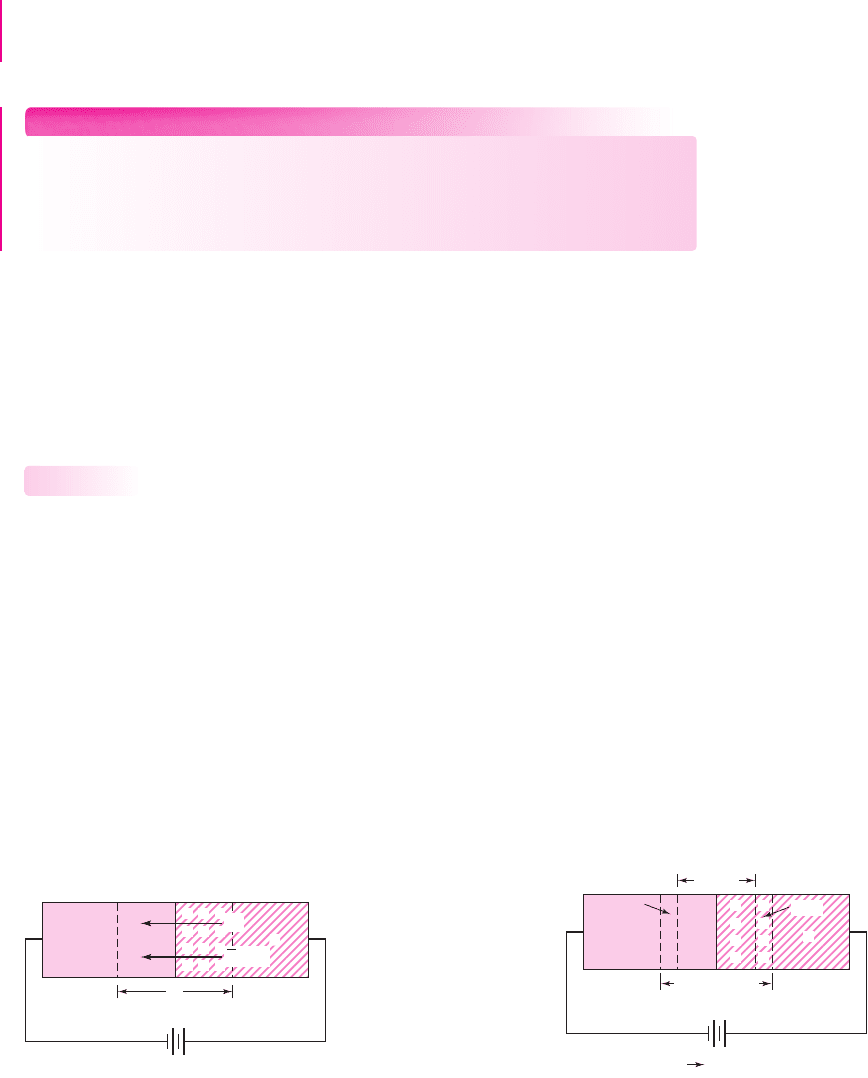
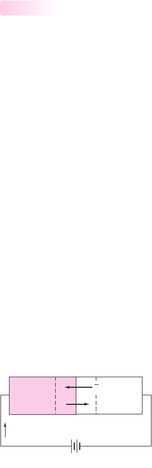
If a positive voltage v

is applied to the p-region, the potential barrier de-

creases (Figure 1.15). The electric ﬁelds in the space-charge region are very large

compared to those in the remainder of the p- and n-regions, so essentially all of the

applied voltage exists across the pn junction region. The applied electric ﬁeld, E

induced by the applied voltage is in the opposite direction from that of the thermal

equilibrium space-charge E-ﬁeld. However, the net electric ﬁeld is always from the

n- to the p-region. The net result is that the electric ﬁeld in the space-charge region

is lower than the equilibrium value. This upsets the delicate balance between dif-

fusion and the E-ﬁeld force. Majority carrier electrons from the n-region diffuse

into the p-region, and majority carrier holes from the p-region diffuse into the n-region.

The process continues as long as the voltage v

is applied, thus creating a current

in the pn junction. This process would be analogous to lowering a dam wall

slightly. A slight drop in the wall height can send a large amount of water (current)

over the barrier.

This applied voltage polarity (i.e., bias) is known as forward bias. The forward-

bias voltage v

must always be less than the built-in potential barrier V

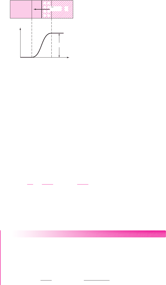
As the majority carriers cross into the opposite regions, they become minority

carriers in those regions, causing the minority carrier concentrations to increase.

Figure 1.16 shows the resulting excess minority carrier concentrations at the space-

charge region edges. These excess minority carriers diffuse into the neutral n- and

p-regions, where they recombine with majority carriers, thus establishing a steady-

state condition, as shown in Figure 1.16.

1.2.3

––

+–

E-field

Figure 1.15 A pn junction with an applied forward-bias voltage showing the direction of

the electric ﬁeld induced by V

and the direction of the original space-charge electric ﬁeld.

The two electric ﬁelds are in opposite directions resulting in a smaller net electric ﬁeld and a

smaller barrier between the p- and n-regions. The net electric ﬁeld is always from the n- to

the p-region.

nea80644_ch01_07-066.qxd 06/08/2009 05:15 PM Page 27 F506 Tempwork:Dont' Del Rakesh:June:Rakesh 06-08-09:MHDQ134-01 Folder:MHDQ134-01: