Patrick F. Dunn, Measurement, Data Analysis, and Sensor Fundamentals for Engineering and Science, 2nd Edition

Подождите немного. Документ загружается.

96 Measurement and Data Analysis for Engineering and Science

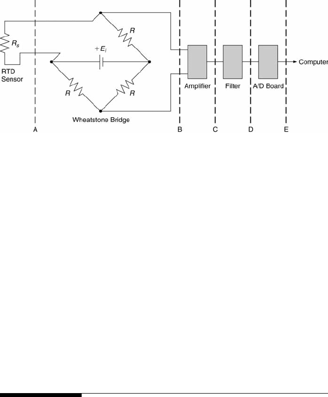
FIGURE 3.25

An example temperature measurement system conﬁguration.

5. A single-stage, low-pass RC ﬁlter with a resistance of 93 Ω is designed

to have a cut-oﬀ frequency of 50 Hz. Determine the capacitance of the

ﬁlter in units of µF.

6. Two resistors, R

and R

, arranged in parallel, serve as the resistance,

, in the leg of a Wheatstone bridge where R

= R

= 200 Ω

and the excitation voltage is 5.0 V. If R

= 1000 Ω, what value of R

is required to give a bridge output of 1.0 V?

7. The number of bits of a 0 V-to-5 V A/D board having a quantization

error of 0.61 mV is (a) 4, (b) 8, (c) 12, (d) 16, or (e) 20.

8. Determine the output voltage, in V, of a Wheatstone bridge having

resistors with resistances of 100 Ω and an input voltage of 5 V.

3.10 Homework Problems

1. Consider the ampliﬁer between stations B and C of the temperature

measurement system shown in Figure 3.25. (a) Determine the minimum

input impedance of the ampliﬁer (in Ω) required to keep the ampliﬁer’s

voltage measurement loading error, e

, less than 1 mV for the case when

the bridge’s output impedance equals 30 Ω and its output voltage equals

0.2 V. (b) Based upon the answer in part (a), if an operational ampliﬁer

were used, would it satisfy the requirement of e

less than 1 mV (Hint:

Compare the input impedance obtained in part (a) to that of a typical

operational ampliﬁer)? Answer yes or no and explain why or why not.

Measurement Systems 97

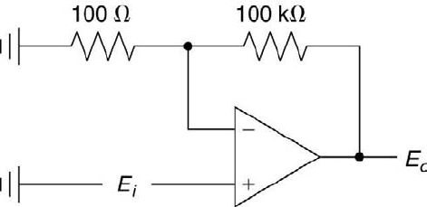
FIGURE 3.26

A closed-loop operational ampliﬁer conﬁguration.

equal to 9 V when T = 72

◦

2. Consider the A/D board between stations D and E of the temperature

measurement system shown in Figure 3.25. Determine how many bits

(M = 4, 8, 12, or 16) would be required to have less than ±0.5 % quan-

tization error for the input voltage of 9 V with E

F SR

= 10 V.

3. The voltage from a 0 kg-to-5 kg strain gage balance scale has a corre-

sponding output voltage range of 0 V to 3.50 mV. The signal is recorded

using a new 16 bit A/D converter having a unipolar range of 0 V to 10 V,

with the resulting weight displayed on a computer screen. An intelligent

aerospace engineering student decides to place an ampliﬁer between the

strain gage balance output and the A/D converter such that 1 % of the

balance’s full scale output will be equal to the resolution of 1 bit of the

converter. Determine (a) the resolution (in mV/bit) of the converter and

(b) the gain of the ampliﬁer.

4. The operational ampliﬁer shown in Figure 3.26 has an open-loop gain

of 10

and an output resistance of 50 Ω. Determine the eﬀective output

resistance (in Ω) of the op amp for the given conﬁguration.

5. A single-stage, passive, low-pass (RC) ﬁlter is designed to have a cut-

oﬀ frequency, f

, of 100 Hz. Its resistance equals 100 Ω. Determine the

ﬁlter’s (a) magnitude ratio at f = 1 kHz, (b) time constant (in ms), and

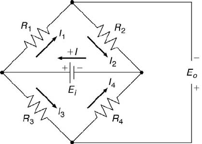
6. A voltage-sensitive Wheatstone bridge (refer to Figure 3.27) is used in

conjunction with a hot-wire sensor to measure the temperature within

a jet of hot gas. The resistance of the sensor (in Ω) is R

= R

[1 +

α(T − T

)], where R

= 50 Ω is the resistance at T

= 0

◦

C and α =

0.00395/

◦

C. For E

= 10 V and R

= R

= 500 Ω, determine (a) the

value of R

(in Ω) required to balance the bridge at T = 0

◦

C. Using

98 Measurement and Data Analysis for Engineering and Science

FIGURE 3.27

The Wheatstone bridge conﬁguration.

this as a ﬁxed R

resistance, further determine (b) the value of R

(in

Ω) at T = 50

◦

C, and (c) the value of E

(in V) at T = 50

◦

C. Next, a

voltmeter having an input impedance of 1000 Ω is connected across the

bridge to measure E

. Determine (d) the percentage loading error in the

measured bridge output voltage. Finally, (e) state what other electrical

component, and in what speciﬁc conﬁguration, could be added between

the bridge and the voltmeter to reduce the loading error to a negligible

value.

7. An engineer is asked to specify several components of a temperature

measurement system. The output voltages from a Type J thermocouple

referenced to 0

◦

C vary linearly from 2.585 mV to 3.649 mV over the

temperature range from 50

◦

C to 70

◦

C. The thermocouple output is to

be connected directly to an A/D converter having a range from −5 V to

+5 V. For both a 12-bit and a 16-bit A/D converter determine (a) the

quantization error (in mV), (b) the percentage error at T = 50

◦

C, and

◦

C. Now if an ampliﬁer is installed

in between the thermocouple and the A/D converter, determine (d) the

ampliﬁer’s gain to yield a quantization error of 5 % or less.

8. Consider the ﬁlter between stations C and D of the temperature mea-

surement system shown in Figure 3.25. Assume that the temperature

varies in time with frequencies as high as 15 Hz. For this condition,

determine (a) the ﬁlter’s cut-oﬀ frequency (in Hz) and (b) the ﬁlter’s

time constant (in ms). Next, ﬁnd (c) the ﬁlter’s output voltage (peak-

to-peak) when the ampliﬁer’s output voltage (peak-to-peak) is 8 V and

the temperature varies with a frequency of 10 Hz and (d) the signal’s

phase lag through the ﬁlter (in ms) for this condition.

Measurement Systems 99

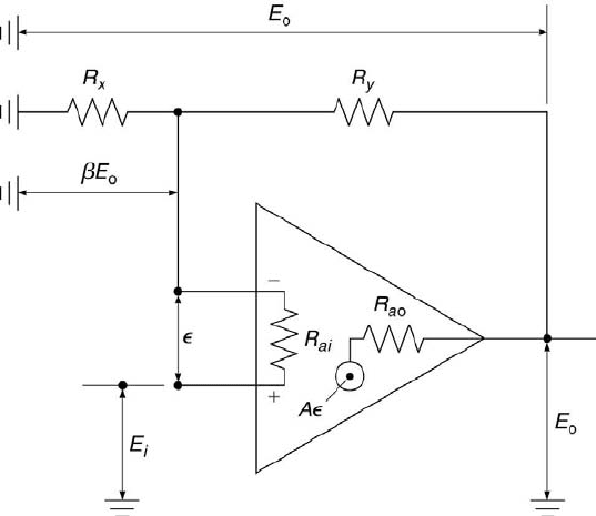
FIGURE 3.28

The operational ampliﬁer in the voltage-follower conﬁguration.

9. An op amp in the negative-feedback, voltage-follower conﬁguration is

shown in Figure 3.28. In this conﬁguration, a voltage diﬀerence, , be-

tween the op amp’s positive and negative inputs results in a voltage

output of A, where A is the open-loop gain. The op amp’s input and

output impedances are R

and R

, respectively. E

is its input volt-

age and E

its output voltage. Assuming that there is negligible current

ﬂow into the negative input, determine (a) the value of β, and (b) the

closed-loop gain, G, in terms of β and A. Finally, recognizing that A is

very large (∼ 10

to 10

), (c) derive an expression for E

as a function

of E

, R

, and R

10. Refer to the information given previously for the conﬁguration shown in

Figure 3.28. When E

is applied to the op amp’s positive input, a current

ﬂows through the input resistance, R

. The op amp’s eﬀective input

resistance, R

, which is the resistance that would be measured between

the op amp’s positive and negative inputs by an ideal ohmmeter, is

deﬁned as E

. (a) Derive an expression for R

as a function of R

β, and A. Using this expression, (b) show that this is a very high value.

11. Refer to the information given previously for the conﬁguration shown in

Figure 3.28. The op amp’s output voltage for this conﬁguration is E

A(E

−βE

). Now assume that there is a load connected to the op amp’s

100 Measurement and Data Analysis for Engineering and Science

output that results in a current ﬂow, I

out

, across the op amp’s output

resistance, R

. This eﬀectively reduces the op amp’s output voltage by

out

. For the equivalent circuit, the Th´evenin output voltage is E

as given in the above expression, and the Th´evenin output impedance

is R

. (a) Derive an expression for R

as a function of R

, β, and A.

Using this expression, (b) show that this is a very low value.

12. A standard RC circuit might be used as a low-pass ﬁlter. If the out-

put voltage is to be attenuated 3 dB at 100 Hz, what should the time

constant, τ, be of the RC circuit to accomplish this?

13. Design an op amp circuit such that the output voltage, E

, is the sum

of two diﬀerent input voltages, E

and E

14. A pitot-static tube is used in a wind tunnel to determine the tunnel’s

ﬂow velocity, as shown in Figure 3.18. Determine the following: (a) the

ﬂow velocity (in m/s) if the measured pressure diﬀerence equals 58 Pa,

(b) the value of R

(in Ω) to have E

= 0 V, assuming R = 100 Ω and

= 200 Ω at a zero ﬂow velocity, with E

= 5.0 V, (c) the value of E

(in V) at the highest ﬂow velocity, at which the parallel combination of

and R

increases by 20 %, (d) the ampliﬁer gain to achieve 80 % of

the full-scale range of the A/D board at the highest ﬂow velocity, (e) the

values of the resistances if the ampliﬁer is a non-inverting operational

ampliﬁer, and (f) the number of bits of the A/D board such that there is

less than 0.2 % error in the voltage reading at the highest ﬂow velocity.

15. A force-balance system comprised of a cantilever beam with four strain

gages has output voltages of 0 mV for 0 N and 3.06 mV for 10 N. The

signal is recorded using a 16-bit A/D converter having a unipolar range

of 0 V to 10 V, with the resulting voltage being displayed on a computer

monitor. A student decides to modify the system to get better force

resolution by installing an ampliﬁer between the force-balance output

and the A/D converter such that 0.2 % of the balance’s output for 10 N

of force will be equal to the resolution of 1 bit of the converter. Determine

(a) the resolution (in mV/bit) of the converter, (b) the gain that the

ampliﬁer must have in the modiﬁed system, and (c) the force (in N) that

corresponds to a 5 V reading displayed on the monitor when using the

modiﬁed system.

Bibliography

[1] R.M. White. 1987. A Sensor Classiﬁcation Scheme. IEEE Transactions

on Ultrasonics, Ferroelectrics and Frequency Control UFFC-34: 124-126.

[2] G.T.A. Kovacs. 1998. Micromachined Transducers Sourcebook. New York:

McGraw-Hill.

[3] J.P. Bentley. 1988. Principles of Measurement Systems. 2nd ed. New

York: John Wiley and Sons.

[4] Wheeler, A.J. and A.R. Ganji. 2004. Introduction to Engineering Exper-

imentation. 2nd ed. New York: Prentice Hall.

[5] E. Doebelin. 2003. Measurement Systems: Application and Design. 5th

ed. New York: McGraw-Hill.

[6] Beckwith, T.G., Marangoni, R.D. and J.H. Leinhard V. 1993. Mechanical

Measurements. 5th ed. New York: Addison-Wesley.

[7] Figliola, R. and D. Beasley. 2000. Theory and Design for Mechanical

Measurements. 3rd ed. New York: John Wiley and Sons.

[8] Alciatore, D.G. and M.B. Histand. 2003. Introduction to Mechatronics

and Measurement Systems. 2nd ed. New York: McGraw-Hill.

[9] Crowe, C., Sommerfeld, M. and Y. Tsuji. 1998. Multiphase Flows with

Droplets and Particles. New York: CRC Press.

[10] T-R. Hsu. 2002. MEMS & Microsystems: Design and Manufacture. New

York: McGraw-Hill.

[11] M. Madou. 1997. Fundamentals of Microfabrication. New York: CRC

Press.

[12] T. Crump, T. 2001. A Brief History of Science as Seen Through the

Development of Scientiﬁc Instruments. London: Robinson.

[13] Horowitz, P. and W. Hill, W. 1989. The Art of Electronics. 2nd ed. Cam-

bridge: Cambridge University Press.

[14] Oppenheim, A.V. and A.S. Willsky. 1997. Signals and Systems. 2nd ed.

New York: Prentice Hall.

101

102 Measurement and Data Analysis for Engineering and Science

[15] T.S. Szarek. 2003. On The Use Of Microcontrollers For Data Acquisi-

tion In An Introductory Measurments Course. M.S. Thesis. Department

of Aerospace and Mechanical Engineering. Indiana: University of Notre

Dame.

Calibration and Response

CONTENTS

4.1 Chapter Overview . . . . . . . . . . . . . . . . . . . . . . . . . . . . . . . . . . . . . . . . . . . . . . . . . . . . . . . . . 103

4.2 Static Response Characterization . . . . . . . . . . . . . . . . . . . . . . . . . . . . . . . . . . . . . . . . . 104

4.3 Dynamic Response Characterization . . . . . . . . . . . . . . . . . . . . . . . . . . . . . . . . . . . . . 106

4.4 Zero-Order System Dynamic Response . . . . . . . . . . . . . . . . . . . . . . . . . . . . . . . . . . . 108

4.5 First-Order System Dynamic Response . . . . . . . . . . . . . . . . . . . . . . . . . . . . . . . . . . . 109

4.5.1 Response to Step-Input Forcing . . . . . . . . . . . . . . . . . . . . . . . . . . . . . . . . . . . 111

4.5.2 Response to Sinusoidal-Input Forcing . . . . . . . . . . . . . . . . . . . . . . . . . . . . . 112

4.6 Second-Order System Dynamic Response . . . . . . . . . . . . . . . . . . . . . . . . . . . . . . . . 118

4.6.1 Response to Step-Input Forcing . . . . . . . . . . . . . . . . . . . . . . . . . . . . . . . . . . . 121

4.6.2 Response to Sinusoidal-Input Forcing . . . . . . . . . . . . . . . . . . . . . . . . . . . . . 123

4.7 Higher-Order System Dynamic Response . . . . . . . . . . . . . . . . . . . . . . . . . . . . . . . . . 125

4.8 *Numerical Solution Methods . . . . . . . . . . . . . . . . . . . . . . . . . . . . . . . . . . . . . . . . . . . . 127

4.9 Problem Topic Summary . . . . . . . . . . . . . . . . . . . . . . . . . . . . . . . . . . . . . . . . . . . . . . . . . 131

4.10 Review Problems . . . . . . . . . . . . . . . . . . . . . . . . . . . . . . . . . . . . . . . . . . . . . . . . . . . . . . . . . . 131

4.11 Homework Problems . . . . . . . . . . . . . . . . . . . . . . . . . . . . . . . . . . . . . . . . . . . . . . . . . . . . . . 133

A single number has more genuine and permanent value than an expensive

library full of hypotheses.

Robert J. Mayer, c. 1840.

Measures are more than a creation of society, they create society.

Ken Alder. 2002. The Measure of All Things. London: Little, Brown.

It is easier to get two philosophers to agree than two clocks.

Lucius Annaeus Seneca, c. 40.

4.1 Chapter Overview

In this chapter, the performance of a measurement system is investigated.

Calibration methods are presented that assure recorded values are accurate

103

104 Measurement and Data Analysis for Engineering and Science

indicators of the variables sensed. Both the static and the dynamic response

characteristics of linear measurement systems are examined. First-order and

second-order systems are considered in detail, including how their output

can lag in time the changes that occur in the experiment’s environment.

With this information, approaches to data acquisition and signal processing,

which are the subjects of subsequent chapters, then can be considered.

4.2 Static Response Characterization

Measurement systems and their instruments are used in experiments to

obtain measurand values that usually are either steady or varying in time.

For both situations, errors arise in the measurand values simply because

the instruments are not perfect; their outputs do not precisely follow their

inputs. These errors can be quantiﬁed through the process of calibration.

In a calibration, a known input value (called the standard) is applied

to the system and then its output is measured. Calibrations can either be

static (not a function of time) or dynamic (both the magnitude and the

frequency of the input signal can be a function of time). Calibrations can be

performed in either sequential or random steps. In a sequential calibration

the input is increased systematically and then decreased. Usually this is

done by starting at the lowest input value and calibrating at every other

input value up to the highest input value. Then the calibration is continued

back down to the lowest input value by covering the alternate input values

that were skipped during the upscale calibration. This helps to identify

any unanticipated variations that could be present during calibration. In a

random calibration, the input is changed from one value to another in no

particular order.

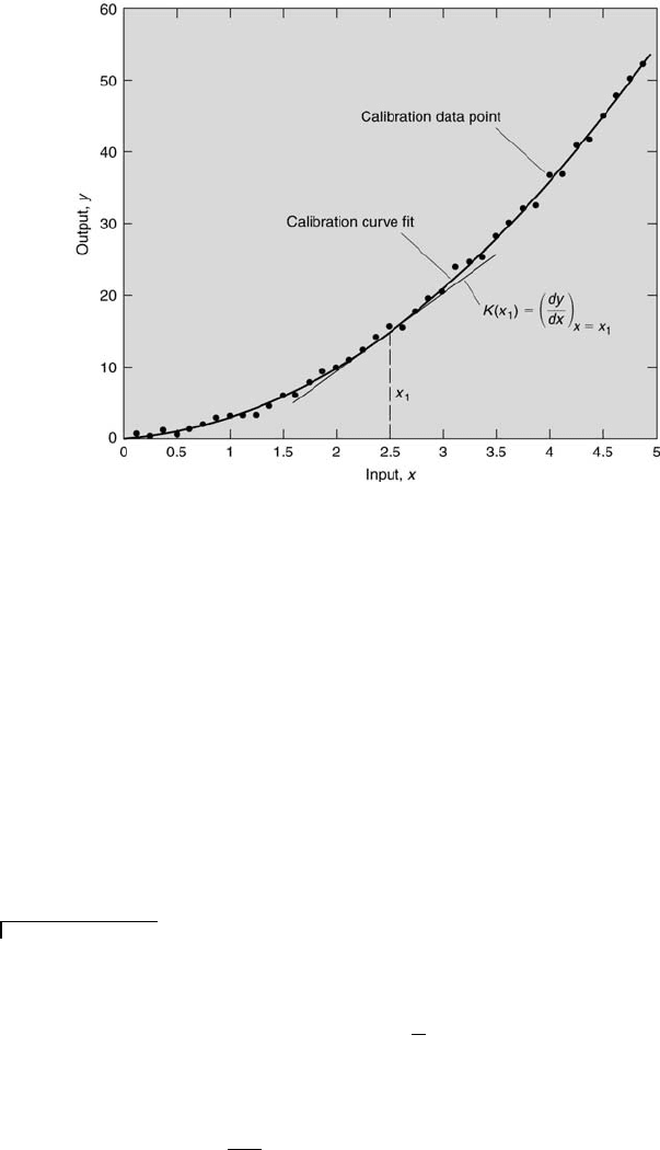
From a calibration experiment, a calibration curve is established. A

generic static calibration curve is shown in Figure 4.1. This curve has several

characteristics. The static sensitivity refers to the slope of the calibration

curve at a particular input value, x

. This is denoted by K, where K =

K(x

) = (dy/dx)

x=x

. Unless the curve is linear, K will not be a constant.

More generally, sensitivity refers to the smallest change in a quantity that

an instrument can detect, which can be determined knowing the value of K

and the smallest indicated output of the instrument. There are two ranges

of the calibration, the input range, x

max

− x

min

, and the output range,

max

− y

min

Calibration accuracy refers to how close the measured value of a calibra-

tion is to the true value. Typically, this is quantiﬁed through the absolute

error, e

abs

, where

abs

= |true value − indicated value|. (4.1)

Calibration and Response 105

FIGURE 4.1

Typical static calibration curve.

The relative error, e

rel

, is

rel

= e

abs

/|true value|. (4.2)

The accuracy of the calibration, a

cal

, is related to the absolute error by

cal

= 1 − e

rel

. (4.3)

Calibration precision refers to how well a particular value is indicated

upon repeated but independent applications of a speciﬁc input value. An

expression for the precision in a measurement and the uncertainties that

arise during calibration are presented in Chapter 7.

Example Problem 4.1

Statement: A hot-wire anemometer system was calibrated in a wind tunnel using a

pitot-static tube. The data obtained is presented in Table 4.1. Using this data, a linear

calibration curve-ﬁt was made, which yielded

= 10.2 + 3.28

√

Determine the following for the curve-ﬁt: [a] the sensitivity, [b] the maximum absolute

error, [c] the maximum relative error, and [d] the accuracy at the point of maximum

relative error.

Solution: Because the curve-ﬁt is linear, the sensitivity of the curve-ﬁt is its slope,

which equals 3.284 V

m/s. The calculated voltages, E

, from the curve-ﬁt expres-

sion are given in Table 4.1. Inspection of the results reveals that the maximum diﬀerence