Patrick F. Dunn, Measurement, Data Analysis, and Sensor Fundamentals for Engineering and Science, 2nd Edition

Подождите немного. Документ загружается.

106 Measurement and Data Analysis for Engineering and Science

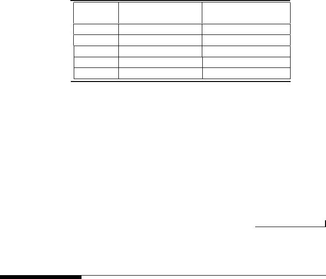
Velocity

Measured voltage

Calculated voltage

U (m/s)

(V)

0.00

3.19

3.05

3.99

6.10

4.30

4.28

9.14

4.48

4.49

12.20

4.65

4.66

TABLE 4.1

Hot-wire anemometer system calibration data.

between the measured and calculated voltages is 0.02 V, which occurs at a velocity of

6.10 m/s. Thus, the maximum absolute error, e

abs

, is 0.02 V, as deﬁned by Equation

4.1. The relative error, e

rel

, is deﬁned by Equation 4.2. This also occurs at a velocity of

6.10 m/s, although maximum relative error does not always occur at the same calibra-

tion point as the maximum absolute error. Here, e

rel

= 0.02/4.30 = 0.01, rounded to

the correct number of signiﬁcant ﬁgures. Consequently, by Equation 4.3, the accuracy

at the point of maximum relative error is 1 − 0.01 = 0.99, or 99 %.

4.3 Dynamic Response Characterization

In reality, almost every measurement system does not respond instanta-

neously to an input that varies in time. Often there is a time delay and

amplitude diﬀerence between the system’s input and output signals. This

obviously creates a measurement problem. If these eﬀects are not accounted

for, dynamic errors will be introduced into the results.

To properly assess and quantify these eﬀects, an understanding of how

measurement systems respond to transient input signals must be gained. The

ultimate goal would be to determine the output (response) of a measurement

system for all conceivable inputs. The dynamic error in the measurement can

be related to the diﬀerence between the input and output at a given time.

In this chapter, only the basics of this subject will be covered. The response

characteristics of several speciﬁc systems (zero, ﬁrst, and second-order) to

speciﬁc transient inputs (step and sinusoidal) will be studied. Hopefully, this

brief foray into dynamic system response will give an appreciation for the

problems that can arise when measuring time-varying phenomena.

First, examine the general formulation of the problem. The output signal,

y(t), in response to the input forcing function of a linear system, F (t), can be

modeled by a linear ordinary diﬀerential equation with constant coeﬃcients

, ..., a

) of the form

Calibration and Response 107

+ a

n−1

+ ... + a

+ a

y = F (t). (4.4)

In this equation n represents the order of the system. The input forcing

function can be written as

F (t) = b

+ b

m−1

+ ... + b

x, m ≤ n, (4.5)

where b

, ..., b

are constant coeﬃcients, x = x(t) is the forcing function, and

m represents its order, where m must always be less than or equal to n to

avoid having an over-deterministic system. By writing F (t) as a polynomial,

the ability to describe almost any shape of forcing function is retained.

The output response, y(t), actually represents a physical variable fol-

lowed in time. For example, it could be the displacement of the mass of an

accelerometer positioned on a ﬂuttering aircraft wing or the temperature

of a thermocouple positioned in the wake of a heat exchanger. The exact

ordinary diﬀerential equation governing each circumstance is derived from a

conservation law, for example, from Newton’s second law for the accelerom-

eter or from the ﬁrst law of thermodynamics for the thermocouple.

To solve for the output response, the exact form of the input forcing

function, F (t), must be speciﬁed. This is done by choosing values for the

, ..., b

coeﬃcients and m. Then Equation 4.4 must be integrated subject

to the initial conditions.

In this chapter, two types of input forcing functions, step and sinusoidal,

are considered for linear, ﬁrst-order, and second-order systems. There are

analytical solutions for these situations. Further, as will be shown in Chap-

ter 9, almost all types of functions can be described through Fourier analysis

in terms of the sums of sine and cosine functions. So, if a linear system’s re-

sponse for sinusoidal-input forcing is determined, then its response to more

complicated input forcing can be described. This is done by linearly su-

perimposing the outputs determined for each of the sinusoidal-input forcing

components that were identiﬁed by Fourier analysis. Finally, note that many

measurement systems are linear, but not all. In either case, the response of

the system almost always can be determined numerically. Numerical solu-

tion methods for such a model will be discussed in Section 4.8.

Now consider some particular systems by ﬁrst specifying the order of

the systems. This is done by substituting a particular value for n into Equa-

tion 4.4.

• For n = 0, a zero-order system is speciﬁed by

y = F (t). (4.6)

108 Measurement and Data Analysis for Engineering and Science

Instruments that behave like zero-order systems are those whose output

is directly coupled to its input. An electrical-resistance strain gage in

itself is an excellent example of a zero-order system, where an input

strain directly causes a change in the gage resistance. However, dynamic

eﬀects can occur when a strain gage is attached to a ﬂexible structure.

In this case the response must be modeled as a higher-order system.

• For n = 1, a ﬁrst-order system is given by

˙y + a

y = F (t). (4.7)

Instruments whose responses fall into the category of ﬁrst-order systems

include thermometers, thermocouples, and other similar simple systems

that produce a time lag between the input and output due to the capacity

of the instrument. For thermal devices, the heat transfer between the

environment and the instrument coupled with the thermal capacitance

of the instrument produces this time lag.

• For n = 2, a second-order system is speciﬁed by

¨y + a

˙y + a

y = F (t). (4.8)

Examples of second-order instruments include diaphragm-type pressure

transducers, U-tube manometers, and accelerometers. This type of sys-

tem is characterized by its inertia. In the U-tube manometer, for exam-

ple, the ﬂuid having inertia is moved by a pressure diﬀerence.

The responses of each of these systems are examined in the following

sections.

4.4 Zero-Order System Dynamic Response

For a zero-order system the equation is

y =





F (t) = KF (t), (4.9)

where K is called the static sensitivity or steady-state gain. It can be seen

that the output, y(t), exactly follows the input forcing function, F (t), in time

and that y(t) is ampliﬁed by a factor, K. Hence, for a zero-order system,

a plot of the output signal values (on the ordinate) versus the input signal

values (on the abscissa) should yield a straight line of slope, K. In fact,

Calibration and Response 109

instrument manufacturers often provide values for the steady-state gains of

their instruments. These values are obtained by performing static calibration

experiments.

4.5 First-Order System Dynamic Response

First-order systems are slightly more complicated. Their governing equation

τ ˙y + y = KF (t), (4.10)

where τ is the time constant of the system = a

. When the time

constant is small, the derivative term in Equation 4.10 becomes negligible

and the equation reduces to that of a zero-order system. That is, the smaller

the time constant, the more instantaneous is the response of the system.

Now digress for a moment and examine the origin of a ﬁrst-order-system

equation. Consider a standard glass bulb thermometer initially at room

temperature that is immersed into hot water. The thermometer takes a

while to read the correct temperature. However, it is necessary to obtain an

equation of the thermometer’s temperature as a function of time after it is

immersed in the hot water in order to be more speciﬁc.

Start by considering the liquid inside the bulb as a ﬁxed mass into which

heat can be transferred. When the thermometer is immersed into the hot

water, heat (a form of energy) will be transferred from the hotter body

(the water) to the cooler body (the thermometer’s liquid). This leads to an

increase in the total energy of the liquid. This energy transfer is governed

by the ﬁrst law of thermodynamics (conservation of energy), which is

, (4.11)

in which E is the total energy of the thermometer’s liquid, Q is the heat

transferred from the hot water to the thermometer’s liquid, and t is time.

The rate at which the heat is transferred into the thermometer’s liquid de-

pends upon the physical characteristics of the interface between the outside

of the thermometer and the hot water. The heat is transferred convectively

to the glass from the hot water and is described by

= hA[T

− T ], (4.12)

where h is the convective heat transfer coeﬃcient, A is the surface area over

which the heat is transferred, and T

is the temperature of the hot water.

Here it is assumed implicitly that there are no conductive heat transfer

losses in the glass. All of the heat transferred from the hot water through

110 Measurement and Data Analysis for Engineering and Science

the glass reaches the thermometer’s liquid. Now as the energy is stored

within the liquid, its temperature increases. For energy within the liquid to

be conserved, it must be that

= mC

, (4.13)

where T is the liquid’s temperature, m is its mass, and C

is its speciﬁc heat

at constant volume.

Thus, upon substitution of Equations 4.12 and 4.13 into Equation 4.11,

= hA[T

− T ]. (4.14)

Rearranging,

+ T = T

. (4.15)

Comparing this equation to Equation 4.10 it can be seen that y = T ,

τ = mC

/hA, and T

= F (t), with K = 1. This is the linear, ﬁrst-order

diﬀerential equation with constant coeﬃcients that relates the time rate of

change in the thermometer’s liquid temperature to its temperature at any

instance of time and the conditions of the situation. Equation 4.15 must be

integrated to obtain the desired equation of the thermometer’s temperature

as a function of time after it is immersed in the hot water.

Another example of a ﬁrst-order system is an electrical circuit comprised

of a resistor of resistance, R, a capacitor of capacitance, C, both in series

with a voltage source with voltage, E

(t). The voltage diﬀerences, ∆V , across

each component in the circuit are ∆V = RI for the resistor and ∆V = Q/C

for the capacitor, where the current, I, is related to the charge, Q, by I =

dQ/dt. Application of Kirchhoﬀ’s voltage law to the circuit gives

+ V = E

(t). (4.16)

Comparing this equation to Equation 4.10 gives τ = RC and K = 1.

Now proceed to solve a ﬁrst-order system equation to determine the

response of the system subject to either a step change in conditions (by

assuming a step-input forcing function) or a periodic change in conditions

(by assuming a sinusoidal-input forcing function). The former, for example,

could be the temperature of a thermometer as a function of time after it is

exposed to a sudden change in temperature, as was examined above. The

latter, for example, could be the temperature of a thermocouple in the wake

behind a heated cylinder.

Calibration and Response 111

4.5.1 Response to Step-Input Forcing

Start by considering the governing equation for a ﬁrst-order system

τ ˙y + y = KF (t), (4.17)

where the step-input forcing function, F (t), is deﬁned as A for t > 0 and

the initial condition y(0) = y

. Equation 4.17 is a linear, ﬁrst-order ordinary

diﬀerential equation. Its general solution (see [24]) is of the form

y(t) = c

+ c

−

. (4.18)

Substitution of this expression for y and the expression for its derivative

˙y into Equation 4.17 yields c

= KA. Subsequently, applying the initial

condition to Equation 4.18 gives c

= y

− KA. Thus, the speciﬁc solution

can be written as

y(t) = KA + (y

− KA) e

−

. (4.19)

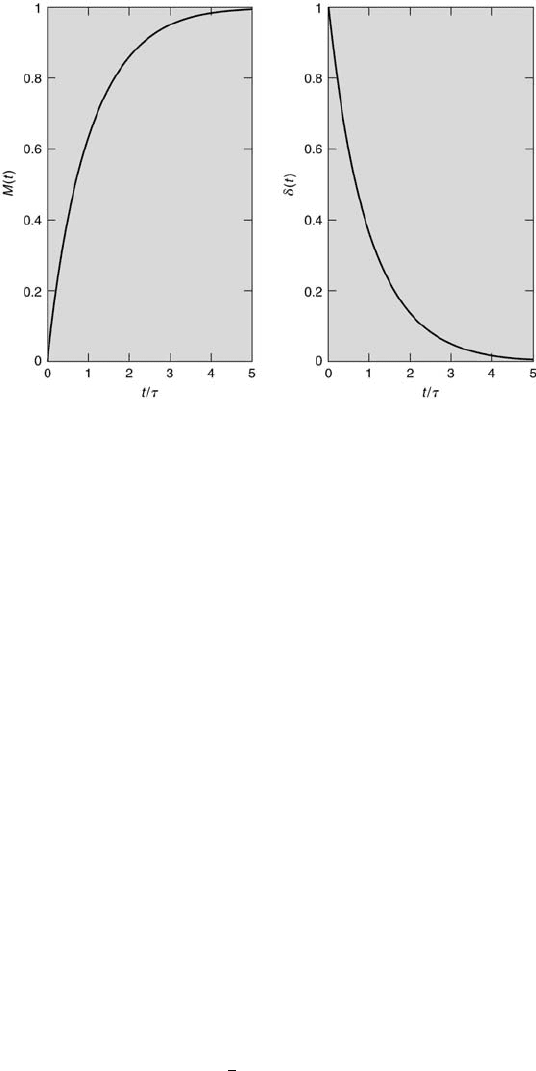
Now examine this equation. When the time equals zero, the exponential

term is unity, which gives y(0) = y

. Also, when time becomes very large

with respect to τ, the exponential term tends to zero, which gives an output

equal to KA. Hence, the output rises exponentially from its initial value

of y

at t = 0 to its ﬁnal value of KA at t >> τ . This is what is seen

in the solution, as shown in the left graph of Figure 4.2. Note that at the

dimensionless time t/τ = 1, the value the signal reaches approximately two-

thirds (actually 1 −

or 0.6321) of its ﬁnal value. The time that it takes

the system to reach 90 % of its ﬁnal value (which occurs at t/τ = 2.303)

is called the rise time of a ﬁrst-order system. At t/τ = 5 the signal has

reached greater than 99 % of its ﬁnal value.

The term y

can be subtracted from both sides of Equation 4.19 and

then rearranged to yield

M(t) ≡

y(t) − y

∞

− y

= 1 − e

−

, (4.20)

noting that y

∞

= KA. M(t) is called the magnitude ratio and is a di-

mensionless variable that represents the change in y at any time t from its

initial value divided by its maximum possible change. When y reaches its

ﬁnal value, M(t) is unity. The right side of Equation 4.20 is a dimensionless

time, t/τ. Equation 4.20 is valid for all ﬁrst-order systems responding to

step-input forcing because the equation is dimensionless.

Alternatively, Equation 4.19 can be rearranged directly to give

y(t) − y

∞

− y

∞

= e

−

≡ δ(t). (4.21)

112 Measurement and Data Analysis for Engineering and Science

FIGURE 4.2

Response of a ﬁrst-order system to step-input forcing.

In this equation δ(t) represents the fractional diﬀerence of y from its ﬁnal

value. This can be interpreted as the fractional dynamic error in y. From

Equations 4.20 and 4.21,

δ(t) = 1 − M(t). (4.22)

This result is plotted in the right graph of Figure 4.2. At the dimensionless

time t/τ = 1, δ equals 0.3678 = 1/e. Further, at t/τ = 5, the dynamic error

is essentially zero (= 0.007). That means for a ﬁrst-order system subjected

to a step change in input it takes approximately ﬁve time constants for

the output to reach the input value. For perfect measurement system there

would be no dynamic error (δ(t) = 0) and the output would always follow

the input [M(t) = 1].

4.5.2 Response to Sinusoidal-Input Forcing

Now consider a ﬁrst-order system that is subjected to an input that varies

sinusoidally in time. The governing equation is

τ ˙y + y = KF (t) = KA sin(ωt), (4.23)

where K and A are arbitrary constants. The units of K would be those of

y divided by those of A. The general solution is

y(t) = y

+ y

= c

−

+ c

sin(ωt) + c

cos(ωt), (4.24)

Calibration and Response 113

in which c

through c

are constants, where the ﬁrst term on the right side

of this equation is the homogeneous solution, y

, and the remaining terms

constitute the particular solution, y

The constants c

through c

can be found by substituting the expressions

for y(t) and its derivative into Equation 4.23. By comparing like terms in

the resulting equation,

= 0, (4.25)

+ 1

, (4.26)

and

= −ωτ C

−ωτKA

+ 1

. (4.27)

The constant c

can be found by applying the initial condition y(0) = y

Equation 4.24, where

= y + 0 − c

ωτKA

+ 1

. (4.28)

Thus, the ﬁnal solution becomes

y(t) = (y

+ ωτ D)e

−

+ D sin(ωt) − ωτ D cos(ωt), (4.29)

where

D =

+ 1

. (4.30)

Now Equation 4.29 can be simpliﬁed further. The sine and cosine terms

can be combined in Equation 4.29 into a single sine term using the trigono-

metric identity

α cos(ωt) + β sin(ωt) =

+ β

sin(ωt + φ), (4.31)

where

φ = tan

−1

(α/β). (4.32)

Equating this expression with the sine and cosine terms in Equation 4.29

gives α = −ωτD and β = D. Thus,

D sin(ωt) − ωτ D cos(ωt) = D

+ 1 =

√

+ 1

(4.33)

and

114 Measurement and Data Analysis for Engineering and Science

φ = tan

−1

(−ωτ) = −tan

−1

(ωτ), (4.34)

or, in units of degrees,

◦

= −(180/π) tan

−1

(ωτ). (4.35)

The minus sign is present in Equations 4.34 and 4.35 by convention to denote

that the output lags behind the input.

The ﬁnal solution is

y(t) = y

+ (

ωτKA

+ 1

−

√

+ 1

sin(ωt + φ). (4.36)

The ﬁrst term on the right side represents the transient response while

the second term is the steady-state response. For ωτ << 1, the transient

term becomes very small and the output follows the input. For ωτ >> 1,

the output is droplets attenuated and its phase is shifted from the input by

φ radians. The phase lag in seconds (lag time), β, is given by

β = φ/ω. (4.37)

Examine this response further in a dimensionless sense. The magnitude

ratio for this input-forcing situation is the ratio of the magnitude of the

steady-state output to that of the input. Thus,

M(ω) =

KA/

√

+ 1

√

+ 1

. (4.38)

The dynamic error, using its deﬁnition in Equation 4.22 and Equation 4.38,

becomes

δ(ω) = 1 −

√

+ 1

. (4.39)

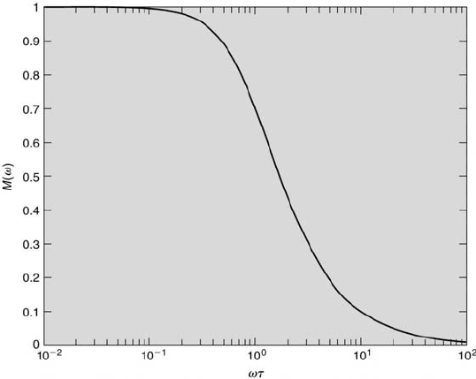
Shown in Figures 4.3 and 4.4, respectively, are the magnitude ratio and

the phase shift plotted versus the product ωτ. First examine Figure 4.3. For

values of τω less than approximately 0.1, the magnitude ratio is very close

to unity. This implies that the system’s output closely follows its input in

this range. At ωτ equal to unity, the magnitude ratio equals 0.707, that is,

the output amplitude is approximately 71 % of its input. Here, the dynamic

error would be 1 − 0.707 = 0.293 or approximately 29 %. Now look at

Figure 4.4. When ωτ is unity, the phase shift equals −45

◦

. That is, the

output signal lags the input signal by 45

◦

or 1/8th of a cycle.

The magnitude ratio often is expressed in units of decibels, abbreviated

as dB. The decibel’s origin began with the introduction of the Bel, deﬁned

in terms of the ratio of output power, P

, to the input power, P

, as

Bel = log

). (4.40)

Calibration and Response 115

FIGURE 4.3

The magnitude ratio of a ﬁrst-order system responding to sinusoidal-input

forcing.

To accommodate the large power gains (output/input) that many systems

had, the decibel (equal to 10 Bels) was deﬁned as

Decibel = 10 log

). (4.41)

Equation 4.41 is used to express sound intensity levels, where P

corresponds

to the sound intensity and P

to the reference intensity, 10

−12

W/m

, which

is the lowest intensity that humans can hear. The Saturn V on launch has

a sound intensity of 172 dB; human hearing pain occurs at 130 dB; a soft

whisper at a distance of 5 m is 30 dB.

There is one further reﬁnement in this expression. Power is a squared

quantity, P

= Q

and P

= Q

, where Q

and Q

are the base measur-

ands, such as volts for an electrical system. With this in mind, Equation 4.41

becomes

Decibel = 10 log

)

= 20 log

). (4.42)

Equation 4.42 is the basic deﬁnition of the decibel as used in measure-

ment engineering. Finally, Equation 4.42 can be written in terms of the

magnitude ratio

dB = 20 log

M(ω). (4.43)