Quinn J.J., Yi K.-S. Solid State Physics: Principles and Modern Applications
Подождите немного. Документ загружается.


Uncorrected Proof
BookID 160928 ChapID 11 Proof# 1 - 29/07/09
334 11 Many Body Interactions – Introduction
Let us consider a most general component of A(r,t)andφ(r,t) 420
A(r,t)=A(q,ω)e
iωt−iq·r
,
φ(r,t)=φ(q,ω)e
iωt−iq·r
.
(11.130)
Thus, we have
421
H
1
=
e
c
A(q,ω) ·
1
2
v
0
e
−iq·r
+e
−iq·r
v
0
− eφ(q,ω)e
−iq·r
e
iωt
. (11.131)
Define the operator V
q
by 422
V
q
=
1
2
v
0
e
iq·r
+
1
2
e
iq·r
v
0
. (11.132)
Then, the matrix element of H
1
can be written 423
k|H
1
|k
=
e
c
A(q,ω) ·k|V
−q
|k
−eφ(q,ω)k|e
−iq·r
|k
. (11.133)
We want to know the charge and current densities at a position r
0
at time t. 424
We can write 425
j(r
0
,t)=Tr
−e
1
2
vδ(r −r
0
)+
1
2
δ(r − r
0
)v
ˆρ
,
n(r
0
,t)=Tr[−eδ(r − r
0
)ˆρ] .
(11.134)
426
Here, −e
1
2
vδ(r −r
0
)+
1
2
δ(r − r
0
)v
is the operator for the current density 427
at position r
0
, while −eδ(r − r
0
) is the charge density operator. The velocity 428
operator v =
1
m
(p +
e
c
A)=v
0
+
e
mc
A is the velocity operator in the presence 429
of the self-consistent field. Because v
0
=
p
m
contains the differential operator 430
−
i¯h
m
∇, it is important to express operator like v
0
e
iq·r
and v
0
δ(r − r
0
)inthe 431
symmetric form to make them Hermitian operators. 432
It is easy to see that 433
j(r
0
,t)=−
e
2
mc
k
k|A(r,t)δ(r −r
0
)ˆρ
0
|k
−e
k
k|
1
2
v
0
δ(r − r
0
)+
1
2
δ(r − r
0
)v
0
ˆρ
1
|k.
(11.135)
δ(r − r
0
) can be written as 434
δ(r − r
0
)=Ω
−1
q
e
iq·(r−r
0
)
. (11.136)
It is clear that k|A(r,t)δ(r − r
0
)ρ
0
|k =Ω
−1
A(r
0
,t)f
0
(ε
k
). Here, of course, 435
Ω is the volume of the system. For j(r
0
,t)weobtain 436
j(r
0
,t)=−
e
2
n
0
mc
A(r
0
,t) −
e
Ω
k,k
,q
k
|V
q
|ke
−iq·r
0
k|ˆρ
1
|k
. (11.137)

Uncorrected Proof
BookID 160928 ChapID 11 Proof# 1 - 29/07/09
11.5 Linear Response Theory 335
But we know the matrix element k|ρ
1
|k
from (11.129). Taking the Fourier 437
transform of j(r
0
,t)gives 438
j(q,ω)= −
e
2
n
0
mc
A(q,ω)−
e
2
Ωc
k,k
f
0
(ε
k
)−f
0
(ε
k
)
ε
k
−ε
k
−¯hω
k
|V
q
|kk|V
q
|k
·A(q,ω)
+
e
2
Ω
k,k
f
0
(ε
k
) − f
0
(ε
k
)
ε
k
− ε
k
− ¯hω
k
|V
q
|kk
|e
iq·r
|k.
(11.138)
This equation can be written as
439
j(q,ω)=−
ω
2
p
4πc
[(1 + I
) ·A(q,ω)+Kφ(q,ω)] . (11.139)
440
Here, ω
2
p
=
4πn
0
e
2
m
is the plasma frequency of the electron gas whose density 441
is n
0
=
N
Ω
,and1 is the unit tensor. The tensor I(q,ω) and the vector K(q,ω) 442
are given by 443
I(q,ω)=
m
N
k,k
f
0
(ε
k
) − f
0
(ε
k
)
ε
k
− ε
k
− ¯hω
k
|V
q
|kk
|V
q
|k
∗
,
K(q,ω)=
mc
N
k,k
f
0
(ε
k
) − f
0
(ε
k
)
ε
k
− ε
k
− ¯hω
k
|V
q
|kk
|e
iq·r
|k.
(11.140)
444
For the plane wave wave functions |k =Ω
−1/2
e
ik·r
the matrix elements are 445
easily evaluated 446
k
|e
iq·r
|k = δ
k
,k+q
,
k
|V
q
|k =
¯h
m
k +
q
2
δ
k
,k+q
.
(11.141)
11.5.7 Gauge Invariance
447
The transformations 448
A
= A + ∇χ = A − iqχ
φ
= φ −
1
c
˙χ = φ − i
ω
c
χ
(11.142)
leave the fields E and B unchanged. Therefore, such a change of gauge must
449
leave j unchanged. Substitution into the expression for j gives the condition 450
(1 + I) · (−iq)+K(−i
ω
c
)=0, or q + I
· q +
ω
c
K =0. (11.143)
Clearly no generality is lost by choosing the z-axis parallel to q. Then, because
451
the summand is an odd function of k
x
or k
y
we have 452
I
xz
= I
zx
= I
yz
= I
zy
= I
xy
= I
yx
= K
x
= K
y
=0. (11.144)

Uncorrected Proof
BookID 160928 ChapID 11 Proof# 1 - 29/07/09
336 11 Many Body Interactions – Introduction
Thus, two of the three components of the relation 453
q + I ·q +
ω
c
K =0
hold automatically. It remains to be proven that
454
q + I
zz
q +
ω
c
K
z
= 0 (11.145)
We demonstrate this by writing I
zz
and K
z
in the following form 455
I
zz
=
¯h
2
mN
(
k
−
f
0
(ε
k
)
ε
k+q
− ε
k
− ¯hω
k
z
+
q
2
2
+
k
f
0
(ε
k+q
)
ε
k+q
− ε
k
− ¯hω
k
z
+
q
2
2
'
(11.146)
In the second term, let k + q =
˜
k so that k =
˜
k − q; then let the dummy
456
variable
˜
k equal −k to have 457
f
0
(ε
k+q
)
ε
k+q
− ε
k
− ¯hω
k
z
+
q
2
2
→
f
0
(ε
k
)
ε
k
− ε
k+q
− ¯hω
−k
z
−
q
2
2
.
With this replacement qI
zz
can be written 458
qI
zz
= −
¯h
2
mN
k
f
0
(ε
k
)
k
z
+
q
2
2
q
ε
k+q
− ε
k
− ¯hω
+
q
ε
k+q
− ε
k
+¯hω
.
(11.147)
Do exactly the same for K
z
to get 459
ω
c
K
z
=
1
N
k
f
0
(ε
k
)
k
z
+
q
2
¯hω
ε
k+q
− ε
k
− ¯hω
−
¯hω
ε
k+q
− ε
k
+¯hω
.
(11.148)
Adding qI
zz
to
ω
c
K
z
gives 460
qI
zz
+
ω
c
K
z
= −
1
N
k
f
0
(ε
k
)
k
z
+
q
2
¯h
2
m
q(k
z
+ q/2) − ¯hω
ε
k+q
− ε
k
− ¯hω
+
¯h
2
m
q(k
z
+ q/2) + ¯hω
ε
k+q
− ε
k
+¯hω
(11.149)
But ε
k+q
−ε
k
=
¯h
2
m
q(k
z
+ q/2), therefore the term in square brackets is equal 461
to 2, and hence we have 462
qI
zz
+
ω
c
K
z
= −
1
N
k
f
0
(ε
k
)
k
z
+
q
2
× 2. (11.150)
The first term
k
f
0
(ε
k
)k
z
= 0 since it is an odd function of k
z
. The second 463
term is −
q
N
k
f
0
(ε
k
)=−q.ThisgivesqI
zz
+
ω
c
K
z
= −q, meaning that 464

Uncorrected Proof
BookID 160928 ChapID 11 Proof# 1 - 29/07/09
11.5 Linear Response Theory 337
(11.145) is satisfied and our result is gauge invariant. Because we have estab- 465
lished gauge invariance, we may now choose any gauge. Let us take φ =0; 466
then we have 467
E(q,ω)=−
iω
c
A(q,ω) (11.151)
for the fields having time dependence of e
iωt
. Substitute this for A and obtain 468
j(q,ω)=−
n
0
e
2
mc
i
ω
[1 + I
(q,ω)] ·E(q,ω). (11.152)
We can write this equation as j(q,ω)=σ
(q,ω) · E(q,ω), where σ, the con- 469
ductivity tensor is given by 470
σ(q,ω)=
ω
2
p
4πiω
[1 + I
(q,ω)] . (11.153)
471
Recall that 472
I(q,ω)=
m
N
k,k
f
0
(ε
k
) − f
0
(ε
k
)
ε
k
− ε
k
− ¯hω
k
|V
q
|kk
|V
q
|k
∗
. (11.154)
473
The gauge invariant result
5
474
j(q,ω)=σ(q,ω) · E(q,ω) (11.155)
475
corresponds to a nonlocal relationship between current density and electric 476
field 477
j(r,t)=
d
3
r
σ(r − r
,t) · E(r
,t). (11.156)
This can be seen by simply writing
478
j(q)=
"
d
3
rj(r)e
iq·r
,
σ
(q)=
"
d
3
(r − r
)σ(r − r
)e
iq·(r−r
)
,
E(q)=
"
d
3
r
E(r
)e
iq·r
,
(11.157)
and substituting into (11.155). Ohm’s law j(r)=σ
(r)·E(r), which is the local 479
relation between j(r)andE(r), occurs when σ(q) is independent of q or, in 480
other words, when 481
σ(r − r
)=σ(r)δ(r − r
).
Evaluation of I
(q,ω) 482
We can see by symmetry that I
xx
= I
yy
and I
zz
are the only non-vanishing 483
components of I. The integration over k can be performed to obtain explicit 484
expressions for I
xx
and I
zz
. We demonstrate this for I
zz
485
5
See, for eample, M.P. Greene, H.J. Lee, J.J. Quinn, S. Rodriguez, Phys. Rev.
177, 1019 (1969) for three-dimensional case and K.S. Yi, J.J. Quinn, Phys. Rev.
B 27, 1184 (1983) for quasi two-dimensional case.

Uncorrected Proof
BookID 160928 ChapID 11 Proof# 1 - 29/07/09
338 11 Many Body Interactions – Introduction
I
zz
(q, ω)=
m
N
k
f
0
(ε
k+q
) − f
0
(ε
k
)
ε
k+q
− ε
k
− ¯hω
¯h
2
m
2
k
z
+
q
2
2
. (11.158)
We can actually return to (11.147) and convert the sum over k to an integral
486
to obtain 487
I
zz
(q, ω)=−
¯h
2
mN
L
2π
3
2
d
3
kf
0
(ε
k
)
k
z
+
q
2
2
¯h
2
m
q
k
z
+
q
2
−¯hω
+
k
z
+
q
2
2
¯h
2
m
q
k
z
+
q
2
+¯hω
.
(11.159)
For zero temperature, f
0
(ε
k
)=1ifk<k
F
and zero otherwise. This gives 488
I
zz
(q, ω)=−
1
4π
2
n
0
q
k
F
−k
F
dk
z
(k
2
F
−k
2
z
)
k
z
+
q
2
2
1
k
z
+
q
2
−
mω
¯hq
+
1
k
z
+
q
2
+
mω
¯hq
.
(11.160)
It is convenient to introduce dimensionless variables z, x,andu defined by 489
z =
q
2k
F
,x=
k
z
k
F
, and u =
ω
qv
F
. (11.161)
Then, I
zz
can be written 490
I
zz
(z,u)=−
3
8z
1
−1
dx(1 − x
2
)(x + z)
2
1
x + z −u
+
1
x + z + u
. (11.162)
If we define I
n
by 491
I
n
=
1
−1
dxx
n
1
x + z − u
+
1
x + z + u
, (11.163)
then I
zz
can be written 492
I
zz
(z,u)=−
3
8z
−I
4
− 2zI
3
+(1− z
2
)I
2
+2zI
1
+ z
2
I
0
. (11.164)
From standard integral tables one can find
493
dx
x
n
x + a
=
1
n
x
n
−
a
n − 1
x
n−1
+
a
2
n − 2
x
n−2
−···+(−a)
n
ln (x + a).
(11.165)
Using this result to evaluate I
n
and substituting the results into (11.164) we 494
find 495
I
zz
(z,u)=−
1+
3
2
u
2
−
3u
2
8z
#
1 − (z −u)
2
ln
z − u +1
z − u − 1
+
1 − (z + u)
2
ln
z + u +1
z + u − 1
$
. (11.166)
496

Uncorrected Proof
BookID 160928 ChapID 11 Proof# 1 - 29/07/09
11.6 Lindhard Dielectric Function 339
In exactly the same way, one can evaluate I
xx
(= I
yy
)toobtain 497
I
xx
(z,u)=
3
8
z
2
+3u
2
−
5
3
−
3
32z
#
1 − (z −u)
2
ln
z −u +1
z −u − 1
+
1 − (z + u)
2
ln
z + u +1
z + u − 1
$
.
(11.167)
498
11.6 Lindhard Dielectric Function 499
In general the electromagnetic properties of a material can be described by 500
two tensors ε(q,ω)andμ(q,ω), where 501
D(q,ω)=ε(q,ω) · E(q,ω)andH(q,ω)=μ
−1
(q,ω) · B(q,ω). (11.168)
For a degenerate electron gas in the absence of a dc magnetic field ε
(q,ω)and 502
μ(q,ω) will be scalars. In his now classic paper “On the properties of a gas of 503
charged particles”, Jens Lindhard
6
used, instead of ε(q,ω)andμ(q,ω), the 504
longitudinal and transverse dielectric functions defined by 505
ε
(l)
= ε and ε
(tr)
= ε
(l)
+
c
2
q
2
ω
2
1 − μ
−1
. (11.169)
Lindhard found this notation to be convenient because he always worked in
506
the particular gauge in which q · A = 0. In this gauge the Maxwell equation 507
for ∇×B =
1
c
˙
E +
4π
c
(j
ind
+ j
0
) can be written, for the fields of the form 508
e
iωt−iq·r
, 509
− iq × (−iq × A)=
iω
c
E +
4π
c
σ
·E +
4π
c
j
0
. (11.170)
But defining
510
ε =1−
4πi
ω
σ
,
and using E =iqφ −
iω
c
A allows us to rewrite (11.170) as 511
q
2
1 −
ω
2
c
2
q
2
ε
(tr)
A = −
ω
c
ε
(l)
qφ +
4π
c
j
0
. (11.171)
Here,wehavemadeuseofthefactthatε
· q involves only ε
(l)
, while ε · A 512
involves only ε
(tr)
since q · A = 0. If we compare (11.171) with the similar 513
equation obtained from ∇×H =
1
c
˙
D +
4π
c
j
0
when H is set equal to μ
−1
B 514
and D = εE,viz. 515
6
J. Lindhard, Kgl. Danske Videnskab. Selskab, Mat.-Fys. Medd. 28, 8 (1954); ibid.,
27, 15 (1953).

Uncorrected Proof
BookID 160928 ChapID 11 Proof# 1 - 29/07/09
340 11 Many Body Interactions – Introduction
q
2
μ
−1
−
ω
2
c
2
q
2
ε
A = −
ω
c
εqφ +
4π
c
j
0
, (11.172)
we see that
516
ε = ε
(l)
and μ
−1
−
ω
2
c
2
q
2
ε
(l)
=1−
ω
2
c
2
q
2
ε
(tr)
. (11.173)
This last equation is simply rewritten
517
ε
(tr)
= ε
(l)
+
c
2
q
2
ω
2
1 − μ
−1
. (11.174)
We have chosen q to be in the z-direction, hence
518
ε
(l)
=1−
4πi
ω
σ
zz
and ε
(tr)
=1−
4πi
ω
σ
xx
. (11.175)
Thus, we have
519
ε
(l)
(q, ω)=1−
ω
2
p
ω
2
[1 + I
zz
(q, ω)]
ε
(tr)
(q, ω)=1−
ω
2
p
ω
2
[1 + I
xx
(q, ω)].
(11.176)
520
11.6.1 Longitudinal Dielectric Constant 521
It is quite apparent from the expression for I
zz
that ε
(l)
has an imaginary 522
part, because for certain values of z and u, the arguments appearing in the 523
logarithmic functions in I
zz
are negative. Recall that 524
ln(x +iy)=
1
2
ln(x
2
+ y
2
)+iarctan
y
x
. (11.177)
One can write ε
(l)
= ε
(l)
1
+iε
(l)
2
. It is not difficult to show that 525
ε
(l)
2
=3u
2
ω
2
p
ω
2
×
⎧
⎨
⎩
π
2
u for z + u<1
π
8z
1 − (z −u)
2
for |z − u| < 1 <z+ u
0for|z − u| > 1
(11.178)
The correct sign of ε
(l)
2
can be obtained by giving ω a small positive imaginary 526
part (then e
iωt
→ 0ast →∞) which allows one to go to zero after evaluation 527
of ε
(l)
2
.Themeaningofε
(l)
2
is not difficult to understand. Suppose that an 528
effective electric field of the form 529
E = E
0
e
−iωt+iq·r
+c.c. (11.179)
perturbs the electron gas. We can write E = −∇φ and then φ
0
=
iE
0
q
.The 530
perturbation acting on the electrons is H
= −eφ. The power (dissipated 531
in the system of unit volume) involving absorption or emission processes of 532
Uncorrected Proof
BookID 160928 ChapID 11 Proof# 1 - 29/07/09
11.6 Lindhard Dielectric Function 341
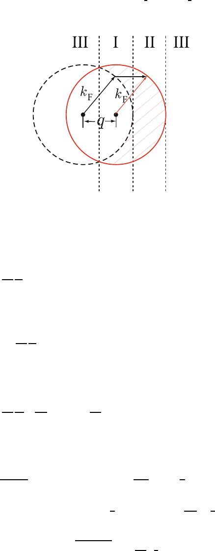
Fig. 11.6. Region of the integration indicated in (11.184)
energy ¯hω is given by P(q,ω)=¯hωW (q,ω). Here, W (q,ω) is the transition 533
rate per unit volume, which is given by the standard Fermi golden rule. Then, 534
we can write the absorption power by 535
P(q,ω)=
2π
¯h
1
Ω
k<k
F
k
>k
F
k
|−eφ
0
e
iq·r
|k
2
¯hω δ(ε
k
− ε
k
− ¯hω). (11.180)
This results in
536
P(q,ω)=
2π
¯h
1
Ω
k<k
F
|k + q| >k
F
e
2
|φ
0
|
2
¯hω δ(ε
k+q
− ε
k
− ¯hω). (11.181)
Now, convert the sums to integrals to obtain
537
P(q,ω)=
2π
¯h
e
2
Ω
E
0
q
2
¯hω 2
L
2π
3
d
3
kδ(ε
k+q
− ε
k
− ¯hω). (11.182)
The prime in the integral denotes the conditions k<k
F
and |k + q| >k
F
(see 538
Fig. 11.6). Now, write
"
d
3
k =
"
dk
z
d
2
k
⊥
.Thus 539
P(q,ω)=
e
2
ωE
2
0
2π
2
q
2
k<k
F
|k + q| >k
F
dk
z
d
2
k
⊥
δ
¯h
2
q
m
k
z
+
q
2
− ¯hω
. (11.183)
Integrating over k
z
and using δ(ax)=
1
a
δ(x)givesk
z
=
mω
¯hq
−
q
2
so that 540
P(q,ω)=
me
2
ωE
2
0
2π¯h
2
q
3
k
z
=
mω
¯hq
−
q
2
d
2
k
⊥
. (11.184)
Uncorrected Proof
BookID 160928 ChapID 11 Proof# 1 - 29/07/09
342 11 Many Body Interactions – Introduction
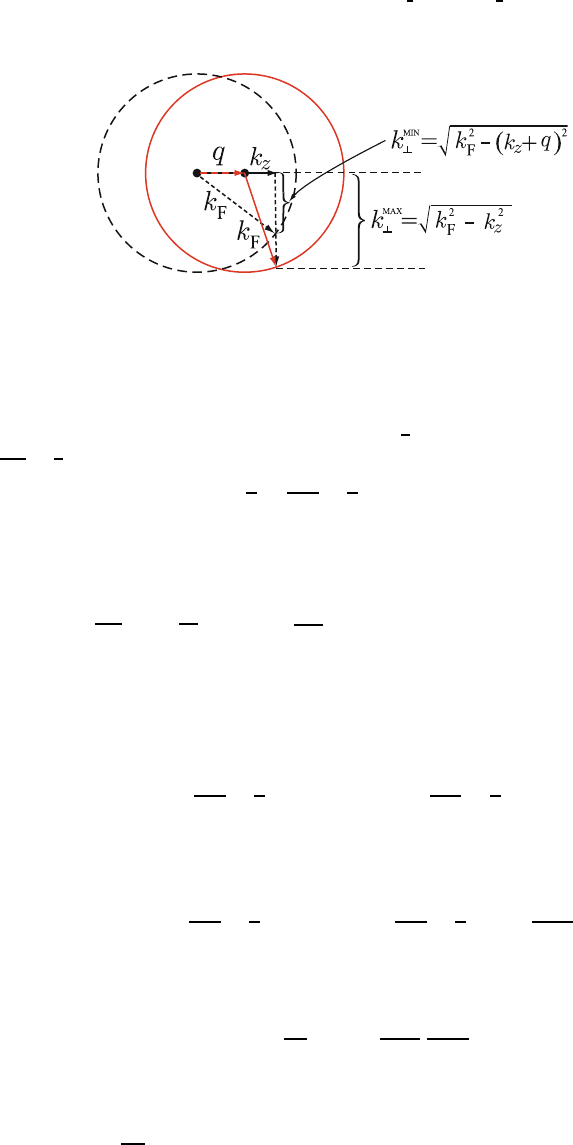
Fig. 11.7. Range of the values of k
⊥
appearing in (11.184)
The solid sphere in Fig. 11.6 represents |k| = k
F
. The dashed sphere has 541
|k−q| = k
F
. Only electrons in the hatched region can be excited to unoccupied 542
states by adding wave vector q to the initial value of k. We divide the hatched 543
region into part I and part II. In region I, −
q
2
<k
z
<k
F
− q,wherek
z
= 544
mω
¯hq
−
q
2
.Thus 545
−
q
2
<
mω
¯hq
−
q
2
<k
F
− q. (11.185)
Divide (11.185) by k
F
to obtain 546
−z<u− z<1 − 2z,
where z =
q
2k
F
,x=
k
z
k
F
, and u =
ω
qv
F
.Now,add2z to each term to have 547
z<u+ z<1oru + z<1. (11.186)
In this region, the values of k
⊥
must be located between the following limits 548
(see Fig. 11.7): 549
k
2
F
−
mω
¯hq
+
q
2
2
<k
2
⊥
<k
2
F
−
mω
¯hq
−
q
2
2
.
550
Therefore, we have 551
d
2
k
⊥
=
k
2
F
−
mω
¯hq
−
q
2
2
−
k
2
F
−
mω
¯hq
+
q
2
2
=
2mω
¯h
. (11.187)
Substituting into (11.184) gives
552
P(q,ω)=
ω
2π
| E
0
|
2
me
2
¯h
2
q
3
2mω
¯h
. (11.188)
Here, we recall that energy dissipated per unit time in the system of vol-
553
ume Ω is also given by E =
"
Ω
j · E d
3
r =2σ
1
(q,ω)|E
0
|
2
Ω and we have that 554
ε(q, ω)=1+
4πi
ω
σ(q, ω) following the form e
−iωt
for the time dependence of 555

Uncorrected Proof
BookID 160928 ChapID 11 Proof# 1 - 29/07/09
11.6 Lindhard Dielectric Function 343
Fig. 11.8. Frequency dependence of ε
(l)
2
(ω) the imaginary part of the dielectric
function
the fields. The power dissipation per unit volume is then written 556
P(q,ω)=
ω
2π
ε
2
(q, ω) | E
0
|
2
. (11.189) 557
We note that ε
2
(q,ω), the imaginary part of the dielectric function determines 558
the energy dissipation in the matter due to a field E of wave vector q and 559
frequency ω. By comparing (11.188) and (11.189), we see that, for region I, 560
ε
(l)
2
(q, ω)=
3ω
2
p
q
2
v
2
F
π
2
u if u + z<1. (11.190)
In region II, k
F
− q<k
z
<k
F
.Butk
z
=
mω
¯hq
−
q
2
= k
F
(u − z). Combining 561
these and dividing by k
F
we have 1 − 2z<u− z<1. Because z<1in 562
region II, the conditions can be expressed as | z −u |< 1 <z+ u.Inthiscase 563
0 <k
2
⊥
<k
2
F
− k
2
z
, and, of course, k
z
= k
F
(u − z). Carrying out the algebra 564
gives for region II 565
ε
(l)
2
(q, ω)=
3ω
2
p
q
2
v
2
F
π
8z
1 − (z −u)
2
if | z − u |< 1 <z+ u. (11.191)
For region III, it is easy to see that ε
(l)
2
(ω) = 0. Figure 11.8 shows the frequency 566
dependence of ε
(l)
2
(ω). Thus, we see that the imaginary part of the dielectric 567
function ε
(l)
2
(q, ω) is proportional to the rate of energy dissipation due to an 568
electric field of the form E
0
e
−iωt+iq·r
+c.c.. 569
11.6.2 Kramers–Kronig Relation 570
Let E(x,t) be an electric field acting on some polarizable material. The polar- 571
ization field P(x,t) will, in general, be related to E by an integral relationship 572
of the form 573