Schneider P., Eberly D.H. Geometric Tools for Computer Graphics
Подождите немного. Документ загружается.

404 Chapter 10 Distance in 3D
P
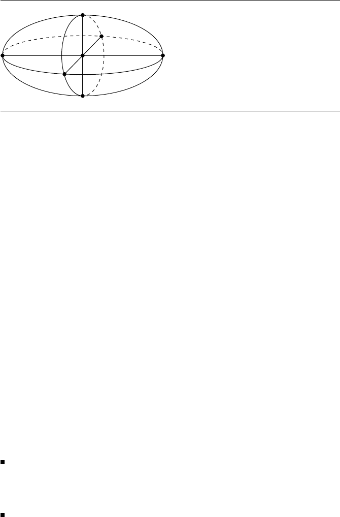
Figure 10.24 Six possible “closest points” on an ellipsoid’s surface.
z
6
(b − c)
2
(b + c)
2
(a −c)
2
(a +c)
2
+ z
5
2c
2
P
z
(b − c)(b + c)(a −c)(a +c)(b
2
+ a
2
− 2c
2
)
+ z
4
− c
2
(−2a
4
b
2
c
2
− 6c
6
P
2
z
+ 6c
4
P
2
z
b
2
+ a
4
b
4
− a
4
c
2
P
2
z
+ c
4
b
4
− 2c
6
b
2
− 2a
2
c
2
b
4
− 4c
2
a
2
P
2
z
b
2
− 2a
2
c
6
+ 6c
4
a
2
P
2
z
+ c
8
+ a
4
c
4
+ 4a
2
c
4
b
2
+ 2c
2
a
2
P
2
x
b
2
− c
4
P
2
y
b
2
− a
4
P
2
y
b
2
− c
2
P
2
z
b
4
− b
4
P
2
x
a
2
− c
4
a
2
P
2
x
+ 2c
2
b
2
P
2
y
a
2
) + z
3
− 2c
4
P
z
(−c
2
b
4
+ c
2
P
2
y
b
2
+ 2c
4
P
2
z
− 4a
2
b
2
c
2
+ 3b
2
c
4
− 2c
6
− c
2
P
2
z
b
2
− b
2
P
2
x
a
2
+ 3c
4
a
2
− a
2
P
2
y
b
2
+ b
2
a
4
− a
4
c
2
− c
2
a
2
P
2
z
+ c
2
a
2
P
2
x
+ b
4
a
2
) + z
2
− c
6
P
2
z
(4a
2
b
2
− 6a
2
c
2
− c
2
P
2
z
− 6b
2
c
2
− P
2
y
b
2
− P
2
x
a
2
+ 6c
4
+ a
4
+ b
4
)
+ z
1
− 2c
8
P
3
z
(b
2
+ a
2
− 2c
2
) + z
0
− c
1
0P
4
z
= 0
Alternatively, consider if P is at the center of the ellipsoid, as shown in Figure 10.24;
there are six candidates at which we must look, at least two of which will have minimal
distance.
In any case, Hart (1994) makes several observations:
The graph of λ has a decreasing slope beyond the largest root. This suggests that
the expensive sixth-degree numerical root finder can be avoided, in favor of, say,
Newton iteration; in that case, providing a “sufficiently large” initial estimate will
result in quick convergence.
If P is (exactly) on the surface, or inside the ellipsoid, an initial guess of λ =0 will
work because the maximum root will be less than or equal to zero.
10.6 Point to Polynomial Curve 405
If P is outside the ellipsoid, then a starting value of
λ =P − Omax{a, b, c}
is “sufficiently large” (O is the origin).
10.6
Point to Polynomial Curve
In this section we address the problem of computing the distance from a point to a
polynomial curve in 3D. Without loss of generality, we assume that our curve is a
parametric polynomial curve (e.g., a B
´
ezier curve), which may be piecewise (e.g., a
NURBS curve).
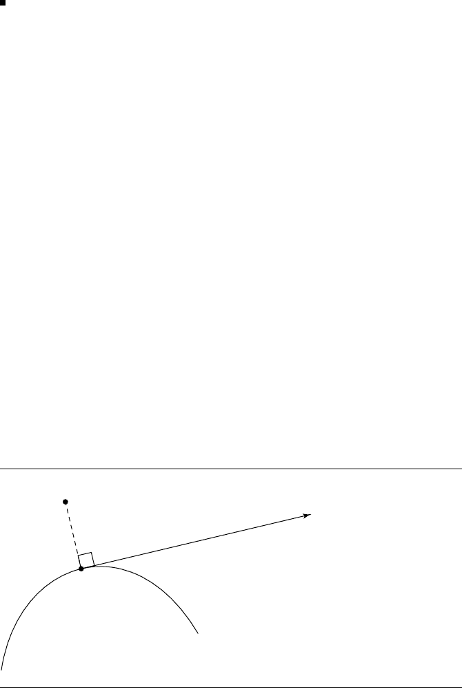
Given a parametric curve Q(t) and a point P , we want to find the point on Q
closest to P . That is, we wish to find the parameter t such that the distance from Q(t)
to P is a minimum. Our approach begins with the geometric observation that the line
segment (whose length we wish to minimize) from P to Q(t) is perpendicular to the
tangent of the curve at Q(t
0
), as shown in Figure 10.25. The equation we wish to solve
for t is
(Q(t) − P)· Q
(t) = 0 (10.10)
If the degree of Q(t ) is d, then Q
(t) is of degree d − 1, so Equation 10.10 is of
degree 2d −1. So, for any curve of degree higher than two, no closed-form solution is
available, and some numerical root finder must be used. One choice is to use Newton
iteration; however, this requires a reasonable first guess. An approach suggested by
P
Q(t)
Q'(t)
Figure 10.25
Distance from an arbitrary point to a parametric curve.

406 Chapter 10 Distance in 3D
Piegl and Tiller (1995) is to evaluate curve points at n equally spaced parameter values
(or at n equally spaced parameter values in the case of a piecewise polynomial curve)
and compute the distance (squared) from each point to P . The parameter value of
the closest evaluated point can be used as the initial guess for the Newton iteration.
Assume we have an initial guess t
0
. Call t
i
the parameter obtained at the ith
Newton iteration. The Newton step is then
t
i+1
= t
i
−
(Q(t) − P)· Q
(t)
(
(Q(t) − P)· Q
(t)
)
= t
i
−
(Q(t) − P)· Q
(t)
(Q(t) − P)· Q
(t
i
) +Q
(t
i
)
2
(10.11)
Newton iteration is, in general, discontinued when some criteria are met. In Piegl
and Tiller (1995), two zero tolerances are used:
1
: a Euclidean distance measure
2
: a zero cosine measure
They check the following criteria in this order:
1. Point coincidence:
Q(t
i
) − P ≤
1
2. Zero cosine (angle between Q(t
i
) − P and Q
(t) is sufficiently close to 90
◦
):
(Q(t) − P)· Q
(t)
Q(t) − P Q
(t)
≤
2
If either of these criteria are not yet met, then a Newton step is taken. Then, two more
conditions are checked:
3. Whether the parameter stays within range a ≤t
i
≤ b by clamping it
4. Whether the parameter doesn’t change significantly:
(t
i+1
− t
i
)Q
(t
i
)≤
1
If the final criterion is satisfied, then Newton iteration is discontinued. The current
parameter value t
i+1
is considered to be the desired root, the closest point to P is
Q(t
i+1
), and the distance from P to the curve Q(t) is (Q(t
i+1
) − P).
An alternative, which avoids the necessity of computing a number of points on
Q(t) required to get a reasonable initial guess for the Newton iteration, is to convert
10.7 Point to Polynomial Surface 407
the curve to B
´
ezier form and use the B
´
ezier-based root finder described in Schneider
(1990); this approach is particularly efficient if the curve is already in B
´
ezier form.
10.7 Point to Polynomial Surface
In this section we address the problem of computing the distance from a point to
a polynomial surface. Without loss of generality, we assume that our surface is a
parametric polynomial surface (e.g., a B
´
ezier surface), which may be piecewise (e.g.,
a NURBS surface).
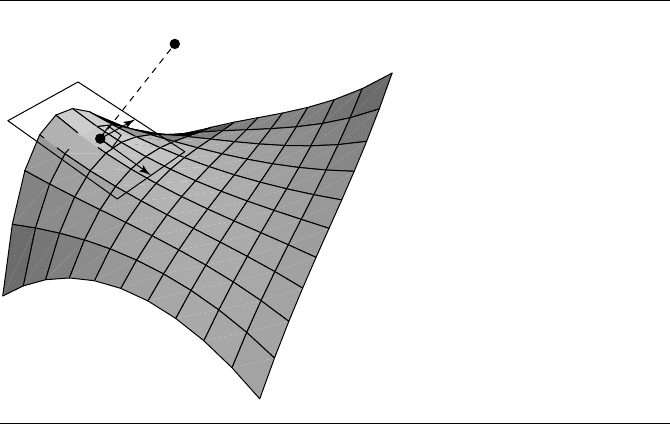
Given a parametric surface S(u, v) and a point P , we want to find the point on S
closest to P . That is, we wish to find the parameters (u, v) such that the distance from
S(u, v) to P is a minimum. Our approach begins with the geometric observation that
the line segment (whose length we wish to minimize) from P to Q(t) is perpendicu-
lar to the tangent plane of the surface at S(u
0
, v
0
), as shown in Figure 10.26.
The vector between the surface and the arbitrary point can be expressed as a
function of the parameters of the surface:
r(u, v) = S(u, v) − P
P
S(u,v)
Figure 10.26 Distance from an arbitrary point to a parametric surface.
408 Chapter 10 Distance in 3D
and the condition for the line S(u, v) − P to be perpendicular to the tangent plane
can be expressed as two conditions—the line must be perpendicular to the partial
derivatives (S
u
(u, v) and S
v
(u, v))ineachdirection:
f(u, v) = r(u, v) · S
u
(u, v)
= 0
g(u, v) = r(u, v) · S
v
(u, v)
= 0
and so in order to find the closest point, we must solve this system of equations. As
with the case of the problem of finding the distance from a point to a polynomial
curve, we use Newton iteration. Again, we can find an initial guess by evaluating the
surface at n × n regularly spaced points, computing the distance (squared) of each
point to P , and using the (u, v) parameters of the closest point as an initial guess for
the Newton iteration.
Let
σ
i
=
δu
δv
=
u
i+1
− u
i
v
i+1
− v
i
J
i
=
f
u
(u
i
, v
i
)f
v
(u
i
, v
i
)
g
u
(u
i
, v
i
)g
v
(u
i
, v
i
)
=
S
u
(u
i
, v
i
)
2
+ r(u
i
, v
i
) · S
uu
(u
i
, v
i
)S
u
(u
i
, v
i
) · S
v
(u
i
, v
i
) + r(u
i
, v
i
) · S
uv
(u
i
, v
i
)
S
u
(u
i
, v
i
) · S
v
(u
i
, v
i
) + r(u
i
, v
i
) · S
vu
(u
i
, v
i
) S
v
(u
i
, v
i
)
2
+ r(u
i
, v
i
) · S
vv
(u
i
, v
i
)
κ
i
=−
f(u
i
, v
i
)
g(u
i
, v
i
)
Assume we have an initial guess of (u
0
, v
0
).Attheith Newton iteration, solve the
2 ×2 system of equations in σ
i
:
J
i
σ
i
= κ
i
and compute the next parameter values as
u
i+1
= δu + u
i
v
i+1
= δv + v
i

10.8 Linear Components 409
Newton iteration is, in general, discontinued when some criteria are met. In Piegl
and Tiller (1995), two zero tolerances are used:
1
: a Euclidean distance measure
2
: a zero cosine measure
They check the following criteria in this order:
1. Point coincidence:
S(u
i
, v
i
) − P ≤
1
2. Zero cosine ((angle between S(u
i
, v
i
) − P and S
u
(u
i
, v
i
) is sufficiently close to
90
◦
, and similarly for S
v
(u
i
, v
i
):
S
u
(u
i
, v
i
) · (S(u
i
, v
i
) − P)
S
u
(u
i
, v
i
)S(u
i
, v
i
) − P
≤
2
S
v
(u
i
, v
i
) · (S(u
i
, v
i
) − P)
S
v
(u
i
, v
i
)S(u
i
, v
i
) − P
≤
2
If either of these criteria are not yet met, then a Newton step is taken. Then, two more
conditions are checked:
3. Whether the parameters stay within range a ≤ u
i
≤b and c ≤v
i
≤d by clamping
them
4. Whether the parameters don’t change significantly:
(u
i+1
− u
i
S
u
(u
i
, v
i
)) + (v
i+1
− v
i
S
u
(u
i
, v
i
))≤
2
10.8
Linear Components
In this section, we discuss the problem of computing the distance between linear
components—lines, segments, and rays—in all combinations.
10.8.1 Lines and Lines
Suppose we have two lines L
0
(s) = P
0
+ s
d
0
and L
1
(t) = P
1
+ t
d
1
, and we wish to
find the minimum distance between them. Let Q
0
= P
0
+ s
c
d
0
and Q
1
= P
1
+ t
c
d
1
be the points on P
0
and P
1
, respectively, such that the distance between them is a
minimum, and let v = Q
0
− Q
1
(see Figure 10.27).

410 Chapter 10 Distance in 3D
d
0
ˆ
P
0
P
1
d
1
ˆ
Q
1
Q
0
v
Figure 10.27 Distance between two lines.
The key to solving the problem of finding s
c
and t
c
(and thereby computing the
minimum distance) is to note that v is perpendicular to both L
0
and L
1
only when
v is minimized. In mathematical terms,
d
0
·v =0 (10.12)
d
1
·v =0 (10.13)
must both be satisfied. If we expand the definition of v:
v = Q
0
− Q
1
= P
0
+ s
c
d
0
− P
1
+ t
c
d
1
and then substitute this back into Equations 10.12 and 10.13, we get
(
d
0
·
d
0
)s
c
− (
d
0
·
d
1
)t
c
=−
d
0
· (P
0
− P
1
)
(
d
1
·
d
0
)s
c
− (
d
1
·
d
1
)t
c
=−
d
1
· (P
0
− P
1
)
Let a =
d
0
·
d
0
, b =−
d
0
·
d
1
, c =
d
1
·
d
1
, d =
d
0
· (P
0
− P
1
), e =
d
1
· (P
0
− P
1
), and
f = (P
0
− P
1
) · P
0
− P
1
). We now have two equations in two unknowns, whose
solution is

10.8 Linear Components 411
s
c
=
be − cd
ac − b
2
t
c
=
bd −ae
ac − b
2
If the denominator ac − b
2
<, then L
0
and L
1
are parallel. In this case, we can
arbitrarily choose t
c
to be anything we like and solve for s
c
. We can minimize the
computations by setting t
c
= 0, in which case the calculation reduces to s
c
=−d/a.
Finally, once we have computed the parameter values of the closest points, we can
compute the distance between L
0
and L
1
:
L
0
(s
c
) − L
1
(t
c
)=(P
0
− P
1
) +
(be − cd)
d
0
− (bd − ae)
d
1
ac − b
2
The pseudocode is
float LineLineDistanceSquared(Line line0, Line line1)
{
u = line0.base - line1.base;
a = Dot(line0.direction, line0.direction);
b = Dot(line0.direction, line1.direction);
c = Dot(line1.direction, line1,direction);
d = Dot(line0.direction, u);
e = Dot(line1.direction, u);
f = Dot(u, u);
det=a*c-b*b;
// Check for (near) parallelism
if (det < epsilon) {
// Arbitrarily choose the base point of line0
s=0;
// Choose largest denominator to minimize floating-point problems
if(b>c){
t=d/b;
} else {
t=e/c;
}
returnd*s+f;
} else {
// Nonparallel lines
invDet=1/det;
s=(b*e-c*d)*invDet;
412 Chapter 10 Distance in 3D
t=(a*e-b*d)*invDet;
returns*(a*s+b*t+2*d)+t*(b*s+c*t+2*e)+f;
}
}
10.8.2 Segment/Segment, Line/Ray, Line/Segment,
Ray/Ray, Ray/Segment
There are three different linear components—lines, rays, and segments—yielding
six different combinations (segment/segment, line/ray, line/segment, ray/ray, ray/
segment, and line/line) for distance tests.
Let’s step back a bit and reconsider the mathematics of the problem at hand. Try-
ing to find the distance between two lines, as we just saw, is equivalent to computing
s and t such that the length of vector v = Q
1
− Q
0
is a minimum. We can rewrite
this as
v
2
=v ·v
= ((P
0
− P
1
) + s
d
0
− t
d
1
) · ((P
0
− P
1
) + s
d
0
− t
d
1
)
This is a quadratic function in s and t; that is, it is a function f(s, t) whose shape
is a paraboloid. For the case of lines, the domain of s and t is unrestricted, and the
solution {s
c
, t
c
}corresponds to the point where f is minimized (that is, the “bottom”
of the paraboloid).
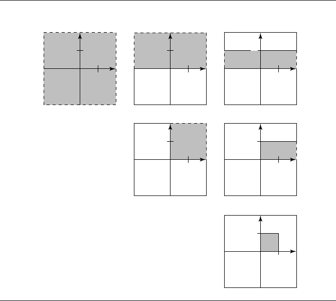
However, if either of the linear components is a ray or line segment, then the
domain of s and/or t is restricted—in the case of a ray, s (or t) must be nonnegative,
and in the case of a line segment, 0 ≤ s ≤1 (and similarly for t). We can create a table
of all the possible combinations of domain restrictions (see Figure 10.28).
In general, the global minimum of the quadratic function may not be within the
restricted domain; in such cases, the minimum will be at some point along oneofthe
boundary edges of the domain. The partitioning of the domain resulting from the re-
striction of the parameter values for either linear component can be used to generate
an algorithm that classifies the location of (s
c
, t
c
), and then applies a “custom” set of
operations to determine the actual closest points and their distance (Section 10.8.3
shows this approach for the intersection of two line segments). However, a somewhat
simpler scheme due to Dan Sunday (2001b) can also be employed.
Analogous to the approach of categorizing the region in which (s
c
, t
c
) lies, this
approach considers which edges of the bounded domain are “visible” to (s
c
, t
c
).For
example, in the case of segment/segment distance, the domain is restricted to [0, 1]×
[0, 1]. Figure 10.29 shows two of the possible visibility conditions for a solution: on
the left, only the boundary t = 1 is visible, and on the right, both s = 1 and t = 1are
visible.
10.8 Linear Components 413
Line
Segment
Line
1
1
s
t
Ray
1
1
s
t
Segment
1
1
s
t
1
1
s
t
Ray
1
1
s
t
1
1
s
t
Figure 10.28 Domains for each possible combination of linear component distance calculation.
By simply comparing the values of s
c
and t
c
, we can easily determine which
domain boundary edges are visible. For each visible boundary edge, we can compute
the point on it closest to (s
c
, t
c
). If only one boundary edge is visible, then that closest
solution point will be in the range [0, 1]; otherwise, the closest solution point will be
outside that range, and thus we need to check the other visible edge.
The basic idea is to first compute the closest points of the infinite lines on which
the ray(s) or segment(s) lie—that is, s
c
and t
c
. If both of these values are within the
domain of the parameters s and t, respectively, of the linear components, then we are
done. However, if one or both the linear components are not infinite lines and are
instead a ray(s) or segment(s), then the domains of s and/or t are restricted, and we
must find the points that minimize the squared-distance function over the restricted
domains; these points will have parameter values that correspond to points on the
boundary.
In Sunday (2001b), we see that we can easily compute the closest points on the
boundary edges by employing a little calculus. For the case of the edge s = 0, we have