Schneider P., Eberly D.H. Geometric Tools for Computer Graphics
Подождите немного. Документ загружается.

474 Chapter 10 Distance in 3D
constraints leads to six polynomial equations in the six unknown components of
X and Y :
ˆn
0
× X = c
0
ˆn
1
× Y = c
1
P
0
(X) = 0
P
1
(Y ) = 0
ˆn
0
×∇P
0
(X) · (X −Y)= 0
ˆn
1
×∇P
1
(Y ) · (Y − X) = 0
As in the case of distance from line to planar curve, the variables may be elimi-
nated directly from the equations to obtain a large-degree polynomial equation in a
single variable. Roots for that equation are found, the remaining five components are
constructed from the various intermediate polynomial equations, and all candidates
X and Y are now known and F is evaluated at those points. The squared distance
between the two curves is the minimum of all such F values.
Smaller-degree polynomial equations may instead be constructed by using the
plane equations to eliminate two variables. That is, if {ˆu
i
, ˆv
i
, ˆn
i
} for i = 0 and i = 1
are two right-handed orthonormal sets, and if C
i
are points on the planes, then
X = C
0
+ u
0
ˆu
0
+ v
0
ˆv
0
and Y =C
1
+ u
1
ˆu
1
+ v
1
ˆv
1
. Replacing these in the other four
constraints leads to four polynomial equations in the four unknowns u
0
, v
0
, u
1
,
and v
1
. The method of elimination applied to these equations yields smaller-degree
polynomials than when applied in terms of the six components of X and Y .
Example Distance between two circles in 3D. For circles in 3D, the polynomials P
0
and P
1
mentioned in the discussion are P
0
(X) =X −C
0
2
−r
2
0
and P
1
(Y ) =Y −C
1
2
−
r
2
1
,whereC
i
are the circle centers and r
i
are the circle radii. The implicit surfaces are
spheres, and their intersection with the planes are circles. From the planar equations,
we can represent X = C
0
+ u
0
ˆu
0
+ v
0
ˆv
0
and Y = C
1
+ u
1
ˆu
1
+ v
1
ˆv
1
. The circles are
defined by u
2
i
+v
2
i
=r
2
i
for i =0, 1. Since ∇P
0
(X) = 2(X − C
0
) = 2r
0
(u
0
ˆu
0
+v
0
ˆv
0
),
the cross product of normal and gradient is ˆn
0
×∇P
0
= 2r
0
(u
0
ˆv
0
− v
0
ˆu
0
).Wehave
made use of the fact that {ˆu
0
, ˆv
0
, ˆn
0
} is a right-handed orthonormal set. Similarly,
ˆn
1
·∇P
1
= 2r
1
(u
1
ˆv
1
− v
1
ˆu
1
). The circle equations and the two equations obtained
from the method of Lagrange multipliers are
u
2
0
+ v
2
0
= r
2
0
u
2
1
+ v
2
1
= r
2
1
(u
0
ˆv
0
− v
0
ˆu
0
) · (C
0
− C
1
− u
1
ˆu
1
− v
1
ˆv
1
) = 0
(u
1
ˆv
1
− v
1
ˆu
1
) · (C
1
− C
0
− u
0
ˆu
0
− v
0
ˆv
0
) = 0
10.13 Miscellaneous 475
a system of four quadratic polynomial equations in the four unknowns u
0
, v
0
, u
1
,
and v
1
.
Setting
ˆ
d = C
0
− C
1
, the last two equations are of the form
u
0
(a
0
+ a
1
u
1
+ a
2
v
1
) + v
0
(a
3
+ a
4
u
1
+ a
5
v
1
) = 0
u
1
(b
0
+ b
1
u
0
+ b
2
v
0
) + v
1
(b
3
+ b
4
u
0
+ b
5
v
0
) = 0
where
a
0
=ˆv
0
·
ˆ
d, a
1
=−ˆv
0
·ˆu
1
, a
2
=−ˆv
0
·ˆv
1
, a
3
=−ˆu
0
·
ˆ
d, a
4
=ˆu
0
·ˆu
1
, a
5
=ˆu
0
·ˆv
1
b
0
=−ˆv
1
·
ˆ
d, b
1
=−ˆv
1
·ˆu
0
, b
2
=−ˆv
1
·ˆv
0
, b
3
=ˆu
1
·
ˆ
d, b
4
=ˆu
1
·ˆu
0
, b
5
=ˆu
1
·ˆv
0
Inmatrixformwehave
m
00
m
01
m
10
m
11
u
0
v
0
=
a
0
+ a
1
u
1
+ a
2
v
1
a
3
+ a
4
u
1
+ a
5
v
1
b
1
u
1
+ b
4
v
1
b
2
u
1
+ b
5
v
1
u
0
v
0
=
0
−(b
0
u
1
+ b
3
v
1
)
=
0
λ
Let M denote the 2 ×2 matrix in the equation. Multiplying by the adjoint of M yields
det(M)
u
0
v
0
=
m
11
−m
01
−m
10
m
00
0
λ
=
−m
01
λ
m
00
λ
(10.17)
Summing the squares of the vector components, using u
2
0
+v
2
0
=r
2
0
, and subtracting
to the left-hand side yields
r
2
0
m
00
m
11
− m
01
m
10
2
−
m
2
00
+ m
2
01
λ
2
= 0 (10.18)
This is a quartic polynomial equation in u
1
and v
1
.
Equation 10.18 can be reduced to a polynomial of degree 8 whose roots v
1
∈
[−1, 1] are the candidates to provide the global minimum of F . Formally comput-
ing the determinant and using u
2
1
= r
2
1
− v
2
1
leads to m
00
m
11
− m
01
m
10
= p
0
(v
1
) +
u
1
p
1
(v
1
),wherep
0
(z) =
2
i=0
p
0i
z
i
and p
1
(z) =
1
i=0
p
1i
z. The coefficients are
p
00
= r
2
1
(a
1
b
2
− a
4
b
1
), p
10
= a
0
b
2
− a
3
b
1
,
p
01
= a
0
b
5
− a
3
b
4
, p
11
= a
1
b
5
− a
5
b
1
+ a
2
b
1
− a
4
b
4
,
p
02
= a
2
b
5
− a
5
b
4
+ a
4
b
1
− a
1
b
2
Similarly, m
2
00
+m
2
01
=q
0
(v
1
) +u
1
q
1
(v
1
),whereq
0
(z) =
2
i=0
q
0i
z
i
and q
1
(z) =
1
i=0
q
1i
z. The coefficients are
476 Chapter 10 Distance in 3D
q
00
= a
2
0
+ a
2
3
+ r
2
1
(a
2
1
+ a
2
4
), q
10
= 2(a
0
a
1
+ a
3
a
4
),
q
01
= 2(a
0
a
2
+ a
3
a
5
), q
11
= 2(a
1
a
2
+ a
4
a
5
),
q
02
= a
2
2
+ a
2
5
− a
2
1
− a
2
4
Finally, λ
2
=r
0
(v
1
) +u
1
r
1
(v
1
),wherer
0
(z) =
2
i=0
r
0i
z
i
and r
1
(z) =
1
i=0
r
1i
z.The
coefficients are
r
00
= r
2
1
b
2
0
, r
10
= 0,
r
01
= 0, r
11
= 2b
0
b
3
,
r
02
= b
2
3
− b
2
0
Replacing p, q, and r in Equation 10.18 and using the identity u
2
1
=1 −v
2
1
yields
0 =r
2
0
[p
0
(v
1
) + u
1
p
1
(v
1
)]
2
− [q
0
(v
1
) + u
1
q
1
(v
1
)][r
0
(v
1
) + u
1
r
1
(v
1
)]
= g
0
(v
1
) + u
1
g
1
(v
1
) (10.19)
where g
0
(z) =
4
i=0
g
0i
z
i
and g
1
(z) =
3
i=0
g
1i
z
i
. The coefficients are
g
00
= r
2
0
(p
2
00
+ r
2
1
p
2
10
) − q
00
r
00
g
01
= 2r
2
0
(p
00
p
01
+ r
2
1
p
10
p
11
) − q
01
r
00
− q
10
r
2
1
r
11
g
02
= r
2
0
(p
2
01
+ 2p
00
p
02
− p
2
10
+ r
2
1
p
2
11
) − q
02
r
00
− q
00
r
02
− r
2
1
q
11
r
11
g
03
= 2r
2
0
(p
01
p
02
− p
10
p
11
) − q
01
r
02
+ q
10
r
11
g
04
= r
2
0
(p
2
02
− p
2
11
) − q
02
r
02
+ q
11
r
11
g
10
= 2r
2
0
p
00
p
10
− q
10
r
00
g
11
= 2r
2
0
(p
01
p
10
+ p
00
p
11
) − q
11
r
00
− q
00
r
11
g
12
= 2r
2
0
(p
02
p
10
+ p
01
p
11
) − q
10
r
02
− q
01
r
11
g
13
= 2r
2
0
p
02
p
11
− q
11
r
02
− q
02
r
11

10.13 Miscellaneous 477
We can eliminate the u
1
term by solving g
0
=−u
1
g
1
, squaring, and subtracting to
the left-hand side to obtain 0 =g
2
0
− (r
2
1
− v
2
1
)g
2
1
= h(v
1
),whereh(z) =
8
i=0
h
i
z
i
.
The coefficients are
h
0
= g
2
00
− r
2
1
g
2
10
h
1
= 2(g
00
g
01
− r
2
1
g
10
g
11
)
h
2
= g
2
01
+ g
2
10
+ 2g
00
g
02
− r
2
1
(g
2
11
+ 2g
10
g
12
)
h
3
= 2(g
01
g
02
+ g
00
g
03
+ g
10
g
11
) − 2r
2
1
(g
11
g
12
+ g
10
g
13
)
h
4
= g
2
02
+ g
2
11
+ 2(g
01
g
03
+ g
00
g
04
+ g
10
g
12
) − r
2
1
(g
2
12
+ 2g
11
g
13
)
h
5
= 2(g
02
g
03
+ g
01
g
04
+ g
11
g
12
+ g
10
g
13
− r
2
1
g
12
g
13
)
h
6
= g
2
03
+ g
2
12
− r
2
1
g
2
13
+ 2(g
02
g
04
+ g
11
g
13
)
h
7
= 2(g
03
g
04
+ g
12
g
13
)
h
8
= g
2
04
+ g
2
13
To find the minimum squared distance, compute all the real-valued roots of
h(v
1
) =0.Foreachroot ¯v
1
∈[−1, 1], compute ¯u
1
=±
1 −¯v
2
1
and choose either (or
both) of these that satisfy Equation 10.19. For each pair ( ¯u
1
, ¯v
1
) solve for ( ¯u
0
, ¯v
0
) in
Equation 10.17. The main numerical issue to deal with is how close to zero is det(M).
Finally, evaluate the squared distance X − Y
2
,whereX = C
0
+¯u
0
ˆu
0
+¯v
0
ˆv
0
and Y =C
1
+¯u
1
ˆu
1
+¯v
1
ˆv
1
. The minimum of all such squared distances is the squared
distance between the circles.
10.13.4 Geodesic Distance on Surfaces
The following discussion can be found in textbooks on the differential geometry of
curves and surfaces. The book by Kay (1988) is a particularly easy one to read. Given
two points on a surface, we want to compute the shortest distance between the two
points measured on the surface. A path of shortest distance connecting the two points
is called a geodesic curve, and the arc length of that curve is called the geodesic distance
between the points. For two points in a plane, the shortest path is the line segment
connecting the points. On a surface, however, it is not necessary that the shortest
path be unique. For example, two antipodal points on a sphere have infinitely many
shortest paths connecting them, each path a half great circle on the sphere.
The method of construction for a geodesic curve that is discussed here is based
on relaxation. Only the ideas are presented since the mathematical details are quite
lengthy. An initial curve connecting the two points and lying on the surface is allowed

478 Chapter 10 Distance in 3D
to evolve over time. The evolution is based on a model of heat flow and has been
studied extensively in the literature under the topic of Euclidean curve shortening.
The ideas also apply to many other areas, particularly to computer vision and image
processing (ter Haar Romeny 1994). The evolving curve is represented as X(s, t),
where s is the arc length parameter and t is the time of evolution. The end points
of the curve are always the two input points, P and Q. In the plane, the idea is
to allow the curve to evolve according to the linear heat equation
X
t
=
X
ss
,where
X
t
is the first-order partial derivative of X with respect to t and
X
ss
is the second-
order partial derivative of X with respect to s. Although X is a point quantity, the
derivatives are vector quantities; hence the use of vector caps on the derivatives. The
limit of the curve as t becomes infinite will be the line segment connecting P and Q.
Any initial curve X(s,0) = C(s) connecting the two points is viewed as a curve that
is “stretched” from its natural state. As time increases, the curve is allowed to “relax”
into its natural state, in this case the line segment connecting the points.
For a surface, the evolution is slightly more complicated:
X
t
=
X
ss
− (
X
ss
·ˆn) ˆn, t>0
X(s,0) =C(s),
X(0, t) = P , X(L(t), t) = Q
(10.20)
The vector ˆn(s, t) is the surface normal at the associated point X(s, t) on the sur-
face. The evolving curve is required to stay on the surface. Any point X(s, t) can only
be moved tangentially to the surface. The movements are determined by the time
derivative
X
t
,so
X
t
must be a tangent vector to the surface. The right-hand side of
the evolution equation has the diffusion term
X
ss
, but observe that the correction
term involving the normal vector simply projects out any contribution by
X
ss
in the
normal direction, leaving only tangential components, as desired. The initial curve
connecting the points is C(s). The length of X(s, t) is denoted by L(t). The bound-
ary conditions are the two constraints that the end points of the curve X(s, t) must
be the points P and Q. This problem is particularly complicated by the time-varying
boundary condition X(L(t), t) =Q. Standard textbooks on partial differential equa-
tions tend to discuss only those problems for which the boundary conditions are time
invariant.
The numerical method for solving the evolution equation, Equation 10.20, uses
a central difference approximation for the s-derivatives and a forward difference
approximation for the t-derivative. That is,
X
ss
(s, t)
.
=
(X(s +h, t) − X(s, t)) + (X(s − h, t) − X(s, t))
h
2

10.13 Miscellaneous 479
and
X
t
(s, t)
.
=
X(s, t + k) − X(s, t)
k
If X(s, t) is known and the surface is defined implicitly by F(X)=0, then the surface
normal at that point is computed explicitly by ˆn(s, t)=∇F(X(s, t))/∇F(X(s, t)).
If the surface is defined parametrically by X(u, v), then the surface normal is
ˆn(u, v) =
X
u
×
X
v
/
X
u
×
X
v
. However, the evolution equation is unaware of the
u and v parameters of the surface, so the normal must be estimated by other means.
As long as the derivatives
X
t
and
X
s
are not parallel (the curve does not stretch only
in the tangent direction during evolution), then the normal vector is estimated as
ˆn(s, t)
.
=
X
s
(s, t) ×
X
t
(s, t)/
X
s
(s, t) ×
X
t
(s, t). Replacing these approximations
in the evolution equation leads to
X(s, t + k) = X(s, t) +
k
h
2
I −ˆn ˆn
T
(
(X(s +h, t) − X(s, t)) + (X(s − h, t) − X(s, t))
)
(10.21)
An initial curve C(s) is chosen, and a set of equally spaced points s
i
,0≤ i ≤ M,
on this curve are selected. The number of chosen points is at the discretion of the
application, but generally the larger the number, the more likely the approximation
to the geodesic curve is a good one. A time step k>0 and spatial step h>0are
chosen. The ratio k/h
2
needs to be sufficiently small to guarantee numerical stability.
How small that is depends on the surface and will require the standard techniques
for determining stability. If X(s
i
,0) = C(s
i
) for all i, the curve samples at time t =k
are computed in the left-hand side X(s
i
, k) of Equation 10.21. Numerical errors can
cause X(s
i
, k) to be off the surface. If the surface is defined implicitly by F(X)= 0,
the defining equation potentially can be used to make a correction to X(s
i
, k) to place
it back on the surface. If the surface is defined parametrically, the correction is a bit
more difficult since it is not immediately clear how to select parameters u and v so
that X(u, v) is somehow the closest surface point to X(s
i
, k).
Equation 10.21 is iterated until some stopping criterion is met. There are many
choices including (1) measuring the total variation between all sample points at times
t and t +k and stopping when the variation is sufficiently small or (2) computing the
arc length of the polyline connecting the samples and stopping when the change in arc
length between times t and t +k is sufficiently small. In either case, the final polyline
arc length is used as the approximation to the geodesic distance.
Chapter
11Intersection
in 3D
This chapter contains information on computing the intersection of geometric prim-
itives in 3D. The simplest object combinations to analyze are those for which one of
the objects is a linear component (line, ray, segment). These combinations are cov-
ered in the first four sections. The next four sections cover intersections of planar
components (planes, triangles, polyhedra) with other objects: one another, polyhe-
dra, quadric surfaces, and polynomial surfaces. Two sections cover the intersection
of quadric surfaces with other quadric surfaces and polynomial surfaces with other
polynomial surfaces. Included is a section covering the method of separating axes,
a very powerful technique for dealing with intersections of convex objects. The last
section covers a miscellany of intersection problems.
11.1 Linear Components and Planar Components
This section covers the problems of computing the intersections of linear compo-
nents and planar components in 3D. Linear components include rays, line segments,
and lines. There are a variety of ways to define such geometric entities (see Sec-
tion 9.1); for the purposes of this section, we use the coordinate-free parametric
representation—a linear component L is defined using a point of origin P and a
direction
d:
L(t) = P + t
d (11.1)
481

482 Chapter 11 Intersection in 3D
ArayR is most frequently defined using a normalized vector
R(t) = P + t
ˆ
d,0≤ t ≤∞ (11.2)
while line L may or may not use a normalized vector:
L(t) = P + t
d, −∞ ≤ t ≤∞ (11.3)
We assume a line segment S is represented by a pair of points {P
0
, P
1
}.Wecan
again employ the same algorithm for ray/planar component intersection by convert-
ing the line segment into ray form:
S(t) = P
0
+ t(P
1
− P
0
)
That is, our direction vector
d is defined by the difference of the two points. Note
that, in general,
d = 1. However, not only is it unnecessary for the direction vector
to be normalized, but it is also undesirable: note that P
1
= P
0
+
d,soifwecompute
the intersection for this “ray” and a planar component, then the point of intersection
is in the line segment if and only if 0 ≤ t ≤ 1.
11.1.1 Linear Components and Planes
In this section, we discuss the problem of intersecting linear components and planes.
A plane P is defined as [
abcd
]:
ax + by + cz + d = 0 (11.4)
where a
2
+ b
2
+ c
2
= 1.Takenasavector, ˆn = [
abc
] represents the normal to
the plane, while |d| represents the minimum distance from the plane to the origin
[
000
].
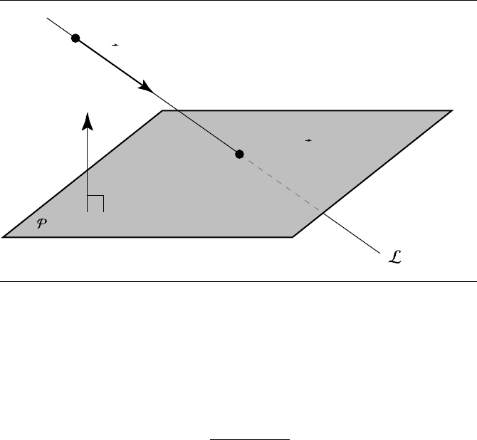
As shown in Figure 11.1, the intersection of the linear component L and P (if it
exists) is at point Q =P +t
d, for some t. Since Q is a point on P, it must also satisfy
Equation 11.4.
We can then simply substitute Equation 11.1 into Equation 11.4:
a
P
x
+ d
x
t
+ b
P
y
+ d
y
t
+ c
P
z
+ d
z
t
+ d = 0
and solve for the parameter t:
t =
−
aP
x
+ bP
y
+ cP
z
+ d
ad
x
+ bd
y
+ cd
z
11.1 Linear Components and Planar Components 483
P
Q = P + td
d
ˆn
Figure 11.1 Intersection of a line and a plane.
It is useful to view this equation as operations on vectors:
t =
−
ˆn · P + d
ˆn ·
d
Note that the denominator ˆn ·
d represents the dot product of the plane’s normal
and the ray’s direction; if this value is equal to 0, then the ray and the plane are
parallel. If the ray is in the plane, then there are an infinite number of intersections,
and if the ray is not in the plane, there are no intersections. Due to the approximate
nature of the floating-point representation of real numbers and operations on them,
lines and planes are rarely ever exactly parallel; thus, the comparison of the dot
product should be made against some small number 0.Thevaluefor0 depends on
the precision of the variables and on application-dependent issues. Calculating this
value first will allow us to quickly reject such cases.
After computing the numerator, we then divide to get t. Computing the inter-
section point’s coordinates requires simply substituting the computed value of t back
into Equation 11.2:
Q = P +t
d