Smith R., Minton R. Calculus
Подождите немного. Документ загружается.

P1: OSO/OVY P2: OSO/OVY QC: OSO/OVY T1: OSO
MHDQ256-Ch01 MHDQ256-Smith-v1.cls December 6, 2010 20:21
LT (Late Transcendental)
CONFIRMING PAGES
1-47 SECTION 1.6
..
Formal Definition of the Limit 93
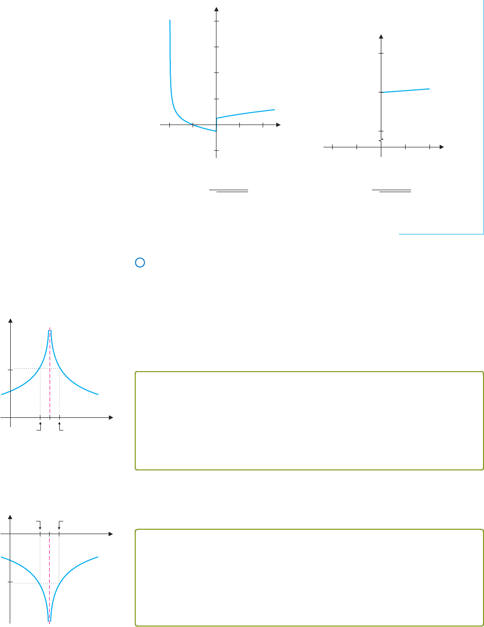
y
x
42
4
2
4
4
8
12
16
x
0.10.1
0.5
1
1.5
y
FIGURE 1.50a
y =
x
2
+ 2x
√
x
3
+ 4x
2
FIGURE 1.50b
y =
x
2
+ 2x
√
x
3
+ 4x
2
You should note here that, while we’ve only shown that the limit is not 1, it’s
somewhat more complicated to show that the limit does not exist.
Limits Involving Infinity
Recall that we write
lim
x→a
f (x) =∞,
whenever the function increases without bound as x → a. That is, we can make f (x)as
large as we like, simply by making x sufficiently close to a. So, given any large positive
number, M, we must be able to make f (x) > M, for x sufficiently close to a. This leads us
to the following definition.
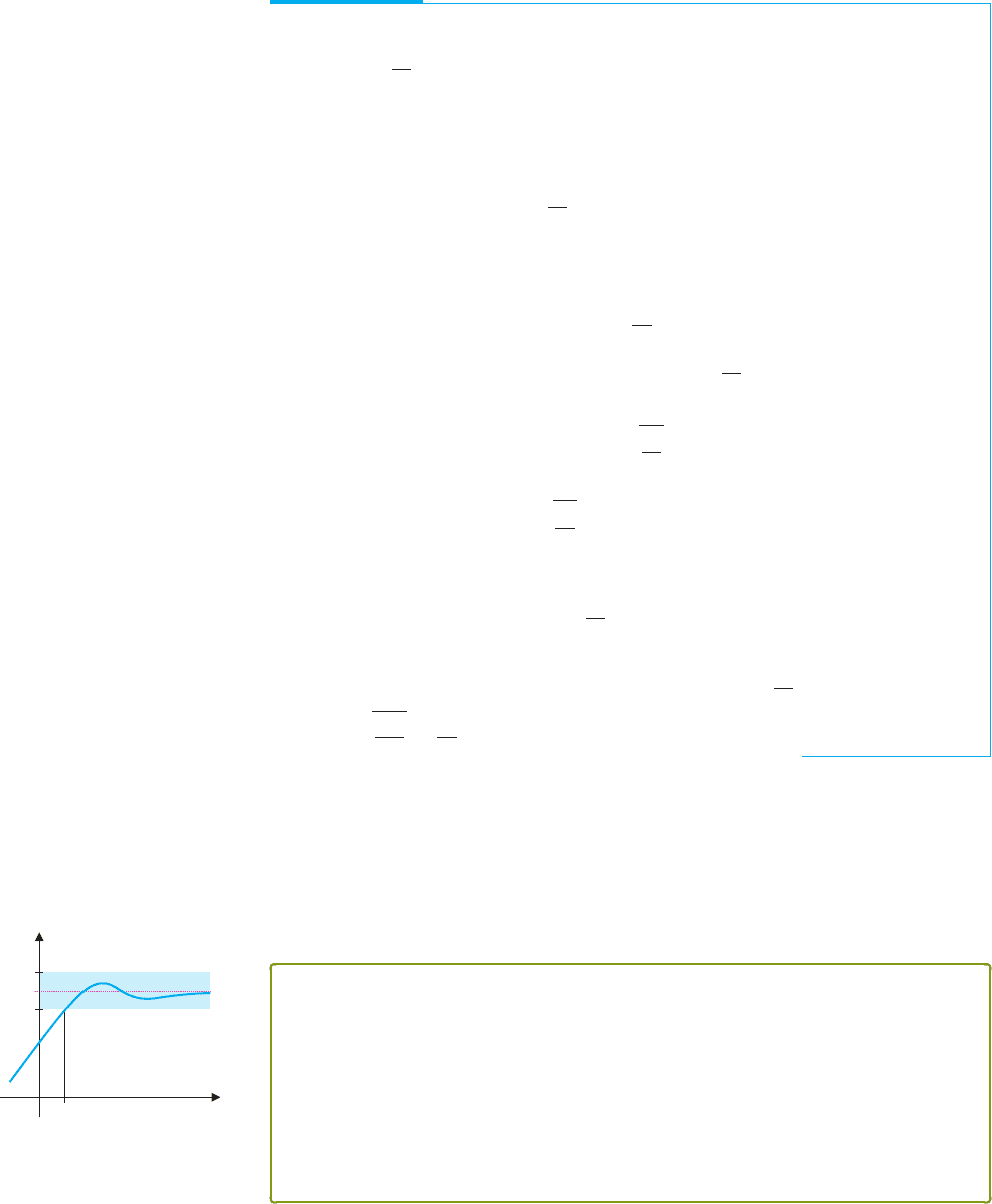
DEFINITION 6.2
For a function f defined in some open interval containing a (but not necessarily at a
itself), we say
lim
x→a
f (x) =∞,
if given any number M > 0, there is another number δ>0, such that 0 < |x −a| <δ
guarantees that f (x) > M. (See Figure 1.51 for a graphical interpretation of this.)
y
x
a
a da d
M
FIGURE 1.51
lim
x→a
f (x) =∞
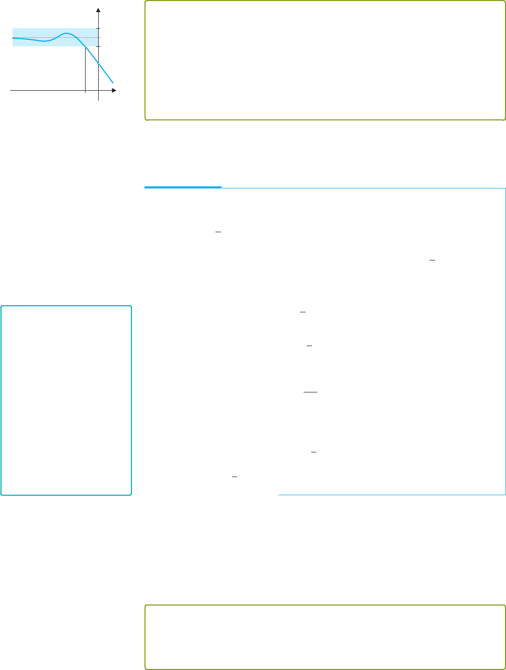
y
x
a
a da d
N
FIGURE 1.52
lim
x→a
f (x) =−∞
Similarly, we had said that if f (x) decreases without bound as x → a, then
lim
x→a
f (x) =−∞. Think of how you would make this more precise and then consider the
following definition.
DEFINITION 6.3
For a function f defined in some open interval containing a (but not necessarily at a
itself), we say
lim
x→a
f (x) =−∞,
if given any number N < 0, there is another number δ>0, such that 0 < |x −a| <δ
guarantees that f (x) < N . (See Figure 1.52 for a graphical interpretation of this.)
It’s easy to keep these definitions straight if you think of their meaning. Don’t simply
memorize them.
P1: OSO/OVY P2: OSO/OVY QC: OSO/OVY T1: OSO
MHDQ256-Ch01 MHDQ256-Smith-v1.cls December 6, 2010 20:21
LT (Late Transcendental)
CONFIRMING PAGES
94 CHAPTER 1
..
Limits and Continuity 1-48
EXAMPLE 6.8 Using the Definition of Limit Where the Limit Is Infinite
Prove that lim
x→0
1
x
2
=∞.
Solution Given any (large) number M > 0, we need to find a distance δ>0 such that
if x is within δ of 0 (but not equal to 0) then
1
x
2
> M. (6.5)
Since both M and x
2
are positive, (6.5) is equivalent to
x
2
<
1
M
.
Taking the square root of both sides and recalling that
√
x
2
=|x|,weget
|x| <
1
M
.
So,forany M > 0,ifwetakeδ =
1
M
andworkbackward,wehavethat0 < |x − 0| <δ
guarantees that
1
x
2
> M,
as desired. Note that this says, for instance, that for M = 100,
1
x
2
> 100, whenever
0 < |x| <
1
100
=
1
10
. (Verify that this works, as an exercise.)
There are two remaining limits that we have yet to place on a careful footing. Before
reading on, try to figure out for yourself what appropriate definitions would look like.
If we write lim
x→∞
f (x) = L, we mean that as x increases without bound, f (x) gets
closer and closer to L. That is, we can make f (x) as close to L as we like, by choosing x
sufficiently large. More precisely, we have the following definition.
M
L
´
y
x
L
L ´
FIGURE 1.53
lim
x→∞
f (x) = L
DEFINITION 6.4
For a function f defined on an interval (a, ∞), for some a > 0, we say
lim
x→∞
f (x) = L,
if given any ε>0, there is a number M > 0 such that x > M guarantees that
| f (x) − L| <ε.
(See Figure 1.53 for a graphical interpretation of this.)
Similarly, we have said that lim
x→−∞
f (x) = L means that as x decreases without bound,
f (x) getscloser and closer to L. So, we shouldbe able to make f (x) as closeto L asdesired,
just by making x sufficiently large in absolute value and negative. We have the following
definition.
P1: OSO/OVY P2: OSO/OVY QC: OSO/OVY T1: OSO
MHDQ256-Ch01 MHDQ256-Smith-v1.cls December 6, 2010 20:21
LT (Late Transcendental)
CONFIRMING PAGES
1-49 SECTION 1.6
..
Formal Definition of the Limit 95
N
y
x
L
´
L
L ´
FIGURE 1.54
lim
x→−∞
f (x) = L
DEFINITION 6.5
For a function f defined on an interval (−∞, a), for some a < 0, we say
lim
x→−∞
f (x) = L,
if given any ε>0, there is a number N < 0 such that x < N guarantees that
| f (x) − L| <ε.
(See Figure 1.54 for a graphical interpretation of this.)
We use Definitions 6.4 and 6.5 essentially the same as we do Definitions 6.1–6.3, as
we see in example 6.9.
EXAMPLE 6.9 Using the Definition of Limit
Where x Tends to −∞
Prove that lim
x→−∞
1
x
= 0.
Solution Here, we must show that given any ε>0, we can make
1
x
within ε of 0,
simply by making x sufficiently large in absolute value and negative. So, we need to
determine those x’s for which
1
x
− 0
<ε
or
1
x
<ε. (6.6)
Since x < 0, |x|=−x and so (6.6) becomes
1
−x
<ε.
Dividing both sides by ε and multiplying by x (remember that x < 0 and ε>0, so
that this will change the direction of the inequality), we get
−
1
ε
> x.
So, if we take N =−
1
ε
and work backward, we have satisfied the definition and thereby
proved that the limit is correct.
REMARK 6.2
You should take care to note
the commonality among the
definitions of the five limits we
have given. All five deal with a
precise description of what it
means to be “close.” It is of
considerable benefit to work
through these definitions until
you can provide your own
words for each. Don’t just
memorize the formal definitions
as stated here. Rather, work
toward understanding what they
mean and come to appreciate
the exacting language that
mathematicians use.
We don’t use the limit definitions to prove each and every limit that comes along.
Actually, we use them to prove only a few basic limits and to prove the limit theorems that
we’ve been using for some time without proof. Further use of these theorems then provides
solid justification of new limits. As an illustration, we now prove the rule for a limit of
a sum.
THEOREM 6.1
Suppose that for a real number a, lim
x→a
f (x) = L
1
and lim
x→a
g(x) = L
2
. Then,
lim
x→a
[ f (x) + g(x)] = lim
x→a
f (x) + lim
x→a
g(x) = L
1
+ L
2
.

P1: OSO/OVY P2: OSO/OVY QC: OSO/OVY T1: OSO
MHDQ256-Ch01 MHDQ256-Smith-v1.cls December 6, 2010 20:21
LT (Late Transcendental)
CONFIRMING PAGES
96 CHAPTER 1
..
Limits and Continuity 1-50
PROOF
Since lim
x→a
f (x) = L
1
, we know that given any number ε
1
> 0, there is a number δ
1
> 0 for
which
0 < |x − a| <δ
1
guarantees that| f (x) − L
1
| <ε
1
. (6.7)
Likewise, since lim
x→a
g(x) = L
2
, we know that given any number ε
2
> 0, there is a number
δ
2
> 0 for which
0 < |x − a| <δ
2
guarantees that|g(x) − L
2
| <ε
2
. (6.8)
Now, in order to get
lim
x→a
[ f (x) + g(x)] = (L
1
+ L
2
),
we must show that, given any number ε>0, there is a number δ>0 such that
0 < |x − a| <δguarantees that|[ f (x) + g(x)] −(L
1
+ L
2
)| <ε.
Notice that
|[ f (x) + g(x)] − (L
1
+ L
2
)|=|[ f (x) − L
1
] + [g(x) − L
2
]|
≤|f (x) − L
1
|+|g(x) − L
2
|, (6.9)
by the triangle inequality. Of course, both terms on the right-hand side of (6.9) can be made
arbitrarily small, from (6.7) and (6.8). In particular, if we take ε
1
= ε
2
=
ε
2
, then as long as
0 < |x − a| <δ
1
and 0 < |x − a| <δ
2
,
we get from (6.7), (6.8) and (6.9) that
|[ f (x) + g(x)] − (L
1
+ L
2
)|≤|f (x) − L
1
|+|g(x) − L
2
|
<
ε
2
+
ε
2
= ε,
as desired. Of course, this will happen if we take
0 < |x − a| <δ= min{δ
1
,δ
2
}.
The other rules for limits are proven similarly. We show these in Appendix A.
EXERCISES 1.6
WRITING EXERCISES
1. In his 1687 masterpiece Mathematical Principles of Natu-
ral Philosophy, which introduces many of the fundamentals
of calculus, Sir Isaac Newton described the important limit
lim
h→0
f (a + h) − f (a)
h
(which we study at length in Chapter 2)
as “the limit to which the ratios of quantities decreasing with-
out limit do always converge, and to which they approach
nearer than by any given difference, but never go beyond,
nor ever reach until the quantities vanish.” If you ever get
weary of all the notation that we use in calculus, think of
what it would look like in words! Critique Newton’s defini-
tion of limit, addressing the following questions in the process.
What restrictions do the phrases “never go beyond” and “never
reach” put on the limit process? Give an example of a simple
limit, not necessarily of the form lim
h→0
f (a + h) − f (a)
h
, that
violates these restrictions. Give your own (English language)
descriptionofthe limit, avoidingrestrictions such asNewton’s.
Why do mathematicians consider the ε−δ definition simple
and elegant?
2. You have computed numerous limits before seeing the def-
inition of limit. Explain how this definition changes and/or
improves your understanding of the limit process.
3. Each word in the ε−δ definition is carefully chosen and pre-
cisely placed. Describe what is wrong with each of the follow-
ing slightly incorrect “definitions” (use examples!):
(a) There exists ε>0 such that there exists a δ>0 such that
if 0 < |x −a| <δ, then | f (x) − L| <ε.
(b) For all ε>0 and for all δ>0, if 0 < |x −a| <δ, then
| f (x) − L| <ε.
(c) For all δ>0 there exists ε>0 such that 0 < |x − a| <δ
and | f (x) − L| <ε.
4. In order for the limit to exist, given every ε>0, we must
be able to find a δ>0 such that the if/then inequalities are
true. To prove that the limit does not exist, we must find a

P1: OSO/OVY P2: OSO/OVY QC: OSO/OVY T1: OSO
MHDQ256-Ch01 MHDQ256-Smith-v1.cls December 6, 2010 20:21
LT (Late Transcendental)
CONFIRMING PAGES
1-51 SECTION 1.6
..
Formal Definition of the Limit 97
particular ε>0 such that the if/then inequalities are not true
for any choice of δ>0. To understand the logic behind the
swapping of the “for every” and “there exists” roles, draw an
analogy with the following situation. Suppose the statement,
“Everybody loves somebody” is true. If you wanted to verify
the statement, why would you have to talk to every person on
earth? But, suppose that the statement is not true. What would
you have to do to disprove it?
In exercises 1–12, symbolically find δ in terms of ε.
1. lim
x→0
3x = 0 2. lim
x→1
3x = 3
3. lim
x→2
(3x + 2) = 8 4. lim
x→1
(3x + 2) = 5
5. lim
x→1
(3 − 4x) =−1 6. lim
x→−1
(3 − 4x) = 7
7. lim
x→1
x
2
+ x − 2
x − 1
= 3 8. lim
x→−1
x
2
− 1
x + 1
=−2
9. lim
x→1
(x
2
− 1) = 0 10. lim
x→1
(x
2
− x + 1) = 1
11. lim
x→2
(x
2
− 1) = 3 12. lim
x→0
(x
3
+ 1) = 1
............................................................
13. Determineaformulaforδ in terms ofε for lim
x→a
(mx + b). (Hint:
Use exercises 1–6.) Does the formula depend on the value of
a? Try to explain this answer graphically.
14. Based on exercises 9 and 11, does the value of δ depend on the
value of a for lim
x→a
(x
2
+ b)? Try to explain this graphically.
............................................................
In exercises 15–18, numerically and graphically determine a δ
corresponding to (a) ε 0.1 and (b) ε 0.05. Graph the func-
tion in the ε − δ window [x-range is (a − δ, a δ) and y-range
is (L − ε, L ε)] to verify that your choice works.
15. lim
x→0
(x
2
+ 1) = 1 16. lim
x→0
cos x = 1
17. lim
x→1
√
x + 3 = 2 18. lim
x→1
x + 2
x
2
= 3
............................................................
19. Modify the ε − δ definition to define the one-sided limits
lim
x→a
−
f (x) and lim
x→a
+
f (x).
20. Symbolically find the largest δ corresponding to ε = 0.1in
the definition of lim
x→1
−
1/x = 1. Symbolically find the largest
δ corresponding to ε = 0.1 in the definition of lim
x→1
+
1/x = 1.
Whichδ couldbeusedinthedefinitionof lim
x→1
1/x = 1?Briefly
explain. Then prove that lim
x→1
1/x = 1.
............................................................
In exercises 21 and 22, find a δ corresponding to M 100 or
N −100 (as appropriate) for each limit.
21. (a) lim
x→1
+
2
x − 1
=∞ (b) lim
x→1
−
2
x − 1
=−∞
22. (a) lim
x→0
+
cot x =∞ (b) lim
x→π
−
cot x =−∞
............................................................
In exercises 23–26, find an M or N corresponding to ε 0.1for
each limit at infinity.
23. lim
x→∞
x
2
− 2
x
2
+ x + 1
= 1 24. lim
x→∞
x
2
+ x
x
2
+ 2x + 1
= 1
25. lim
x→−∞
x
2
+ 3
4x
2
− 4
= 0.25 26. lim
x→−∞
3x
2
− 2
x
2
+ 1
= 3
............................................................
In exercises 27–32, prove that the limit is correct using the ap-
propriate definition (assume that k is an integer).
27. lim
x→∞
1
x
2
+ 2
− 3
=−3 28. lim
x→∞
1
(x − 7)
2
= 0
29. lim
x→−3
−2
(x + 3)
4
=−∞ 30. lim
x→7
3
(x − 7)
2
=∞
31. lim
x→∞
1
x
k
= 0, fork > 0 32. lim
x→−∞
1
x
2k
= 0, fork > 0
............................................................
In exercises 33–36, identify a specific ε>0 for which no δ>0
exists to satisfy the definition of limit.
33. f (x) =
2x if x < 1
,
lim
x→1
f (x) = 2
x
2
+ 3ifx > 1
34. f (x) =
x
2
− 1ifx < 0
,
lim
x→0
f (x) =−2
−x − 2ifx > 0
35. f (x) =
2x if x < 1
,
lim
x→1
f (x) = 2
5 − x
2
if x > 1
36. f (x) =
x − 1ifx < 2
,
lim
x→2
f (x) = 1
x
2
if x > 2
............................................................
37. Prove Theorem 3.1 (i).
38. Prove Theorem 3.1 (ii).
39. Prove the Squeeze Theorem, as stated in Theorem 3.5.
40. Given that lim
x→a
−
f (x) = L and lim
x→a
+
f (x) = L, prove that
lim
x→a
f (x) = L.
41. A metal washer of (outer) radius r inches weighs 2r
2
ounces.
A company manufactures 2-inch washers for different cus-
tomers who have different error tolerances. If the customer
demands a washer of weight 8 ±ε ounces, what is the error
tolerance for the radius? That is, find δ such that a radius of
r within the interval (2 − δ, 2 +δ) guarantees a weight within
(8 − ε,8+ε).
42. A fiberglass company ships its glass as spherical marbles. If
the volume of each marble must be within ε of π/6, how close
does the radius need to be to 1/2?
EXPLORATORY EXERCISES
1. In this section, we have not yet solved any problems we
could not already solve in previous sections. We do so
now, while investigating an unusual function. Recall that
P1: OSO/OVY P2: OSO/OVY QC: OSO/OVY T1: OSO
MHDQ256-Ch01 MHDQ256-Smith-v1.cls December 6, 2010 20:21
LT (Late Transcendental)
CONFIRMING PAGES
98 CHAPTER 1
..
Limits and Continuity 1-52
rational numbers can be written as fractions p/q, where
p and q are integers. We will assume that p/q has been
simplified by dividing out common factors (e.g., 1/2 and
not 2/4). Define f (x) =
0ifx is irrational
1/q if x =
p
q
is rational
.We
will try to show that lim
x→2/3
f (x) exists. Without graphics,
we need a good definition to answer this question. We know
that f (2/3) = 1/3, but recall that the limit is independent of
the actual function value. We need to think about x’s close
to 2/3. If such an x is irrational, f (x) = 0. A simple hy-
pothesis would then be lim
x→2/3
f (x) = 0. We’ll try this out for
ε = 1/6. We would like to guarantee that |f (x)| < 1/6 when-
ever 0 < |x − 2/3| <δ. Well, how many x’s have a function
value greater than 1/6? The only possible function values are
1/5, 1/4, 1/3, 1/2 and 1. The x’s with function value 1/5 are
1/5, 2/5, 3/5, 4/5 and so on. The closest of these x’s to 2/3
is 3/5. Find the closest x (not counting x = 2/3) to 2/3 with
function value 1/4. Repeat for f (x) = 1/3, f (x) = 1/2 and
f (x) = 1. Out of all these closest x’s, how close is the ab-
solute closest? Choose δ to be this number, and argue that if
0 < |x −2/3| <δ, we are guaranteed that | f (x)| < 1/6. Ar-
gue that a similar process can find a δ for any ε.
2. State a definition for “ f (x) is continuous at x = a” using Def-
inition 6.1. Use it to prove that the function in exploratory
exercise 1 iscontinuous at every irrational numberand discon-
tinuous at every rational number.
1.7 LIMITS AND LOSS-OF-SIGNIFICANCE ERRORS
“Pay no attention to that man behind the curtain....” (from The Wizard of Oz)
Things are not always what they appear to be. Even so, people tend to accept a computer’s
answer as a fact not subject to debate. However, when we use a computer (or calculator), we
mustalwayskeepinmindthatthesedevicesperformmostcomputationsonlyapproximately.
Most of the time, this will cause us no difficulty whatsoever. Occasionally, however, the
resultsof round-offerrors ina string of calculations are disastrous. In this section,we briefly
investigate these errors and learn how to recognize and avoid some of them.
We first consider a relatively tame-looking example.
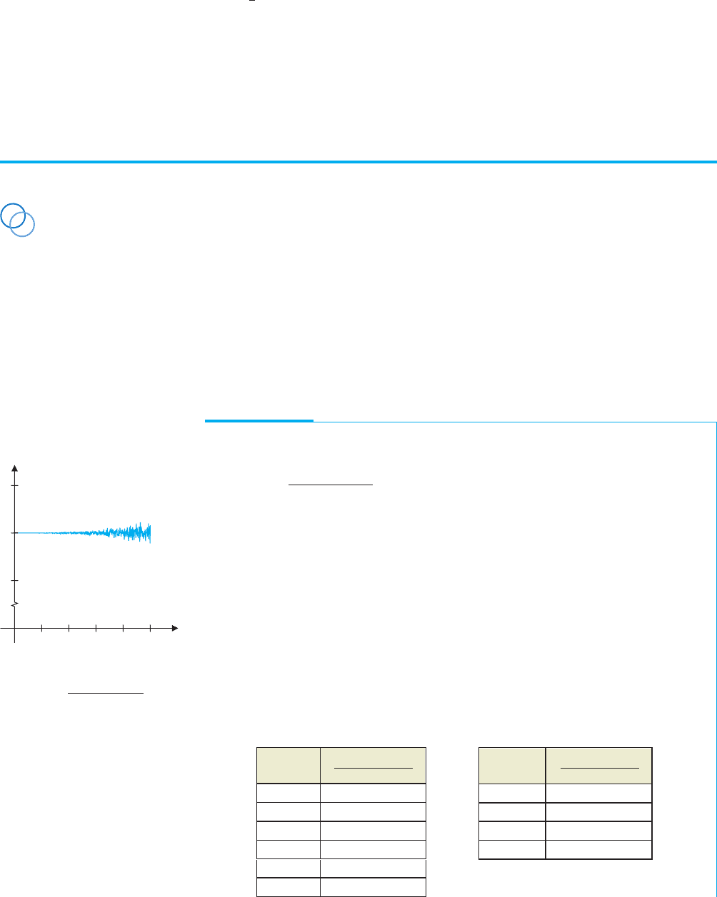
EXAMPLE 7.1 A Limit with Unusual Graphical
and Numerical Behavior
Evaluate lim
x→∞
(x
3
+ 4)
2
− x
6
x
3
.
x
100,00060,00020,000
y
7
8
9
FIGURE 1.55a
y =
(x
3
+ 4)
2
− x
6
x
3
Solution At first glance, the numerator looks like ∞−∞, which is indeterminate,
while the denominator tends to ∞. Algebraically, the only reasonable step is to multiply
out the first term in the numerator. First, we draw a graph and compute some function
values.(Not all computers and software packages will produce these identical results, but
for large values of x,you should see results similar to those shown here.) In Figure 1.55a,
the function appears nearly constant, until it begins oscillating around x = 40,000.
Notice that the accompanying table of function values is inconsistent with Figure 1.55a.
The last two values in the table may have surprised you. Up until that point, the
function values seemed to be settling down to 8.0 very nicely. So, what happened here
and what is the correct value of the limit? To answer this, we look carefully at function
values in the interval between x = 1 × 10
4
and x = 1 ×10
5
. A more detailed table is
shown below to the right.
Incorrect calculated values
x
(x
3
4)
2
− x
6
x
3
10 8.016
100 8.000016
1 × 10
3
8.0
1 × 10
4
8.0
1 × 10
5
0.0
1 × 10
6
0.0
x
(x
3
4)
2
− x
6
x
3
2 × 10
4
8.0
3 × 10
4
8.14815
4 × 10
4
7.8125
5 × 10
4
0
P1: OSO/OVY P2: OSO/OVY QC: OSO/OVY T1: OSO
MHDQ256-Ch01 MHDQ256-Smith-v1.cls December 6, 2010 20:21
LT (Late Transcendental)
CONFIRMING PAGES
1-53 SECTION 1.7
..
Limits and Loss-of-Significance Errors 99
In Figure 1.55b, we have blown up the graph to enhance the oscillation observed
between x = 1 ×10
4
and x = 1 ×10
5
. The deeper we look into this limit, the more
erratically the function appears to behave. We use the word appears because all of the
oscillatory behavior we are seeing is an illusion, created by the finite precision of the
computer used to perform the calculations and draw the graph.
x
100,00060,00020,000
y
7.8
8
8.2
FIGURE 1.55b
y =
(x
3
+ 4)
2
− x
6
x
3
Computer Representation of Real Numbers
Thereasonfortheunusualbehaviorseeninexample7.1boilsdowntothewayinwhichcom-
puters represent real numbers. Without getting into all of the intricacies of computer arith-
metic, it suffices to think of computers and calculators as storing real numbers internally in
scientific notation. For example, the number 1,234,567 would be stored as 1.234567 ×10
6
.
The number preceding the power of 10 is called the mantissa and the power is called the
exponent. Thus, the mantissa here is 1.234567 and the exponent is 6.
All computing devices have finite memory and consequently have limitations on the
size mantissa and exponent that they can store. (This is called finite precision.) Many
calculators carry a 14-digit mantissa and a 3-digit exponent. On a 14-digit computer, this
would suggest that the computer retains only the first 14 digits in the decimal expansion of
any given number.
EXAMPLE 7.2 Computer Representation of a Rational Number
Determinehow
1
3
isstoredinternallyona10-digitcomputerandhow
2
3
isstoredinternally
on a 14-digit computer.
Solution On a 10-digit computer,
1
3
is stored internally as 3.333333333
10digits
×10
−1
.Ona
14-digitcomputer,
2
3
isstored internallyas6.6666666666667
14digits
×10
−1
.
For most purposes, such finite precision presents no problem. However, this occasion-
ally leads to a disastrous error. In example 7.3, we subtract two relatively close numbers
and examine the resulting catastrophic error.
EXAMPLE 7.3 A Computer Subtraction of Two “Close” Numbers
Compare the exact value of
1. 0000000000000
13zeros
4 × 10
18
− 1. 0000000000000
13zeros
1 × 10
18
with the result obtained from a calculator or computer with a 14-digit mantissa.
Solution Notice that
1. 0000000000000
13zeros
4×10
18
−1. 0000000000000
13zeros
1×10
18
= 0. 0000000000000
13zeros
3×10
18
= 30,000.
(7.1)
However, if this calculation is carried out on a computer or calculator with a 14-digit
(or smaller) mantissa, both numbers on the left-hand side of (7.1) are stored by the
computer as 1 × 10
18
and hence, the difference is calculated as 0. Try this calculation
for yourself now.

P1: OSO/OVY P2: OSO/OVY QC: OSO/OVY T1: OSO
MHDQ256-Ch01 MHDQ256-Smith-v1.cls December 6, 2010 20:21
LT (Late Transcendental)
CONFIRMING PAGES
100 CHAPTER 1
..
Limits and Continuity 1-54
EXAMPLE 7.4 Another Subtraction of Two “Close” Numbers
Compare the exact value of
1. 0000000000000
13zeros
6 × 10
20
− 1. 0000000000000
13zeros
4 × 10
20
with the result obtained from a calculator or computer with a 14-digit mantissa.
Solution Notice that
1.0000000000000
13zeros
6×10
20
−1.0000000000000
13zeros
4×10
20
= 0.0000000000000
13zeros
2×10
20
= 2,000,000.
However, if this calculation is carried out on a calculator with a 14-digit mantissa, the
first number is represented as 1.0000000000001 × 10
20
, while the second number is
represented by 1.0 × 10
20
, due to the finite precision and rounding. The difference
between the two values is then computed as 0.0000000000001 ×10
20
or 10,000,000,
which is, again, a very serious error.
In examples 7.3 and 7.4, we witnessed a gross error caused by the subtraction of two
numbers whose significant digits are very close to one another. This type of error is called
a loss-of-significant-digits error or simply a loss-of-significance error. These are subtle,
often disastrous computational errors. Returning now to example 7.1, we will see that it
was this type of error that caused the unusual behavior noted.
EXAMPLE 7.5 A Loss-of-Significance Error
In example 7.1, we considered the function f (x) =
(x
3
+ 4)
2
− x
6
x
3
.
Followthecalculationof f (5 × 10
4
)onestepatatime,asa 14-digitcomputer woulddoit.
Solution We have
f (5 ×10
4
) =
[(5 × 10
4
)
3
+ 4]
2
− (5 ×10
4
)
6
(5 × 10
4
)
3
=
(1.25 × 10
14
+ 4)
2
− 1.5625 ×10
28
1.25 × 10
14
=
(125,000,000,000,000 + 4)
2
− 1.5625 ×10
28
1.25 × 10
14
=
(1.25 × 10
14
)
2
− 1.5625 ×10
28
1.25 × 10
14
= 0,
since 125,000,000,000,004 is rounded off to 125,000,000,000,000.
Note that the real culprit here was not the rounding of 125,000,000,000,004, but the
fact that this was followed by a subtraction of a nearly equal value. Further, note that
this is not a problem unique to the numerical computation of limits.
REMARK 7.1
If at all possible, avoid
subtractions of nearly equal
values. Sometimes, this can be
accomplished by some algebraic
manipulation of the function.
In the case of the function from example 7.5, we can avoid the subtraction and hence,
the loss-of-significance error by rewriting the function as follows:
f (x) =
(x
3
+ 4)
2
− x
6
x
3
=
(x
6
+ 8x
3
+ 16) − x
6
x
3
=
8x
3
+ 16
x
3
,
P1: OSO/OVY P2: OSO/OVY QC: OSO/OVY T1: OSO
MHDQ256-Ch01 MHDQ256-Smith-v1.cls December 6, 2010 20:21
LT (Late Transcendental)
CONFIRMING PAGES
1-55 SECTION 1.7
..
Limits and Loss-of-Significance Errors 101
where we have eliminated the subtraction. Using this new (and equivalent) expression for
the function, we can compute a table of function values reliably. Notice, too, that if we
redraw the graph in Figure 1.55a using the new expression (see Figure 1.56), we no longer
see the oscillation present in Figures 1.55a and 1.55b.
From the rewritten expression, we easily obtain
lim
x→∞
(x
3
+ 4)
2
− x
6
x
3
= 8,
which is consistent with Figure 1.56 and the corrected table of function values.
In example 7.6, we examine a loss-of-significance error that occurs for x close to 0.
x
100,00060,00020,000
y
7
8
9
FIGURE 1.56
y =
8x
3
+ 16
x
3
x
8x
3
16
x
3
10 8.016
100 8.000016
1 × 10
3
8.000000016
1 × 10
4
8.00000000002
1 × 10
5
8.0
1 × 10
6
8.0
1 × 10
7
8.0
EXAMPLE 7.6 Loss-of-Significance Involving
a Trigonometric Function
Evaluate lim
x→0
1 − cos x
2
x
4
.
Solution As usual, we look at a graph (see Figure 1.57) and some function values.
y
x
0.5
2424
FIGURE 1.57
y =
1 − cos x
2
x
4
x
1 − cos x
2
x
4
0.1 0.499996
0.01 0.5
0.001 0.5
0.0001 0.0
0.00001 0.0
x
1 − cos x
2
x
4
−0.1 0.499996
−0.01 0.5
−0.001 0.5
−0.0001 0.0
−0.00001 0.0
As in example 7.1, note that the function values seem to be approaching 0.5, but then
suddenly take a jump down to 0.0. Once again, we are seeing a loss-of-significance
error. In this particular case, this occurs because we are subtracting nearly equal values
(cos x
2
and 1). We can again avoid the error by eliminating the subtraction. Note that
1 − cos x
2
x
4
=
1 − cos x
2
x
4
·
1 + cos x
2
1 + cos x
2
Multiply numerator and
denominator by (1 +cos x
2
).
=
1 − cos
2
x
2
x
4
1 + cos x
2
1 −cos
2
(x
2
) = sin
2
(x
2
).
=
sin
2
x
2
x
4
1 + cos x
2
.
Since this last (equivalent) expression has no subtraction indicated, we should be able to
use it to reliably generate values without the worry of loss-of-significance error. Using
this to compute function values, we get the accompanying table.
Using the graph and the new table, we conjecture that
lim
x→0
1 − cos x
2
x
4
=
1
2
.
x
sin
2
(x
2
)
x
4
(1 cos x
2
)
±0.1 0.499996
±0.01 0.4999999996
±0.001 0.5
±0.0001 0.5
±0.00001 0.5
We offer one final example where a loss-of-significance error occurs, even though no
subtraction is explicitly indicated.
EXAMPLE 7.7 A Loss-of-Significance Error Involving a Sum
Evaluate lim
x→−∞
x[(x
2
+ 4)
1/2
+ x].
P1: OSO/OVY P2: OSO/OVY QC: OSO/OVY T1: OSO
MHDQ256-Ch01 MHDQ256-Smith-v1.cls December 6, 2010 20:21
LT (Late Transcendental)
CONFIRMING PAGES
102 CHAPTER 1
..
Limits and Continuity 1-56
Solution Initially, you might think that since there is no subtraction (explicitly)
indicated, there will be no loss-of-significance error. We first draw a graph (see
Figure 1.58) and compute a table of values.
x x
(x
2
4)
1/2
x
−100 −1.9998
−1 × 10
3
−1.999998
−1 × 10
4
−2.0
−1 × 10
5
−2.0
−1 × 10
6
−2.0
−1 × 10
7
0.0
−1 × 10
8
0.0
y
x
3
2
1
2 10
7
6 10
7
1 10
8
FIGURE 1.58
y = x[(x
2
+ 4)
1/2
+ x]
You should notice the sudden jump in values in the table and the wild oscillation
visible in the graph. Although a subtraction is not explicitly indicated, there is indeed a
subtraction here, since we have x < 0 and (x
2
+ 4)
1/2
> 0. We can again remedy this
with some algebraic manipulation, as follows.
x
(x
2
+ 4)
1/2
+ x
= x
(x
2
+ 4)
1/2
+ x
(x
2
+ 4)
1/2
− x
(x
2
+ 4)
1/2
− x
Multiply numerator and
denominator by the conjugate.
= x
(x
2
+ 4) − x
2
(x
2
+ 4)
1/2
− x
Simplify the numerator.
=
4x
(x
2
+ 4)
1/2
− x
.
We use this last expression to generate a graph in the same window as that used for
Figure 1.58 and to generate the accompanying table of values. In Figure 1.59, we can
see none of the wild oscillation observed in Figure 1.58 and the graph appears to be a
horizontal line.
y
x
3
2
1
2 10
7
6 10
7
1 10
8
FIGURE 1.59
y =
4x
(x
2
+ 4)
1/2
− x
x
4x
(x
2
4)
1/2
− x
−100 −1.9998
−1 × 10
3
−1.999998
−1 × 10
4
−1.99999998
−1 × 10
5
−1.9999999998
−1 × 10
6
−2.0
−1 × 10
7
−2.0
−1 × 10
8
−2.0
Further, the values displayed in the table no longer show the sudden jump indicative of a
loss-of-significance error. We can now confidently conjecture that
lim
x→−∞
x[(x
2
+ 4)
1/2
+ x] =−2.