Smith R., Minton R. Calculus
Подождите немного. Документ загружается.


P1: OSO/OVY P2: OSO/OVY QC: OSO/OVY T1: OSO
MHDQ256-Ch04 MHDQ256-Smith-v1.cls December 13, 2010 21:23
LT (Late Transcendental)
CONFIRMING PAGES
4-3 SECTION 4.1
..
Antiderivatives 253
EXAMPLE 1.1 Finding Several Antiderivatives of a Given Function
Find an antiderivative of f (x) = x
2
.
Solution Notice that F(x) =
1
3
x
3
is an antiderivative of f (x), since
F
(x) =
d
dx
1
3
x
3
= x
2
.
Further, observe that
d
dx
1
3
x
3
+ 5
= x
2
,
so that G(x) =
1
3
x
3
+ 5 is also an antiderivative of f. In fact, for any constant c,wehave
d
dx
1
3
x
3
+ c
= x
2
.
Thus, H(x) =
1
3
x
3
+ c is also an antiderivative of f (x), for any choice of the constant c.
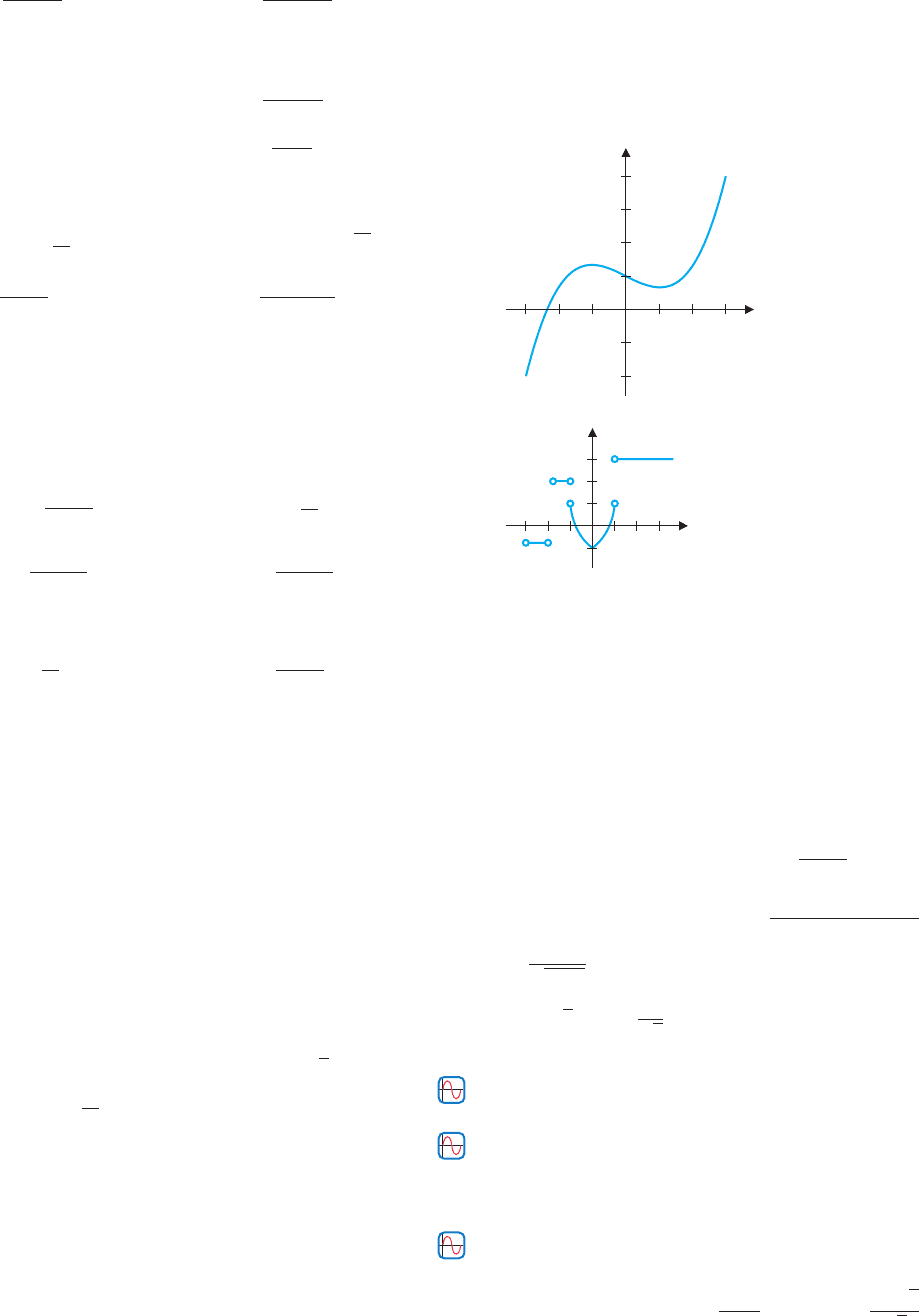
Graphically, this gives us a family of antiderivative curves, as illustrated in Figure 4.1.
Note that each curve is a vertical translation of every other curve in the family.
x
y
−2
−4
−2
2
4
240−4
FIGURE 4.1
A family of antiderivative curves
In general, observe that if F is any antiderivative of f and c is any constant, then
d
dx
[F(x) +c] = F
(x) +0 = f (x).
Thus, F(x) + c is also an antiderivative of f (x), for any constant c. On the other hand,
are there any other antiderivatives of f (x) besides F(x) + c? The answer, as provided in
Theorem 1.1, is no.
THEOREM 1.1
Suppose that F and G are both antiderivatives of f on an interval I . Then,
G(x) = F(x) + c,
for some constant c.
PROOF
Since F and G are both antiderivatives for f, we have that G
(x) = F
(x). It now fol-
lows, from Corollary 8.1 in section 2.8, that G(x) = F(x) + c, for some constant c,
as desired.
DEFINITION 1.1
Let F be any antiderivative of f on an interval I . The indefinite integral of f (x)
(with respect to x)onI is defined by
f (x) dx = F(x) + c,
where c is an arbitrary constant (the constant of integration).
The process of computing an integral is called integration. Here, f (x) is called the inte-
grand and the term dx identifies x as the variable of integration.
NOTES
Theorem 1.1 says that given any
antiderivative F of f, every
possible antiderivative of f can be
written in the form F(x) + c, for
some constant, c. We give this
most general antiderivative a
name in Definition 1.1.

P1: OSO/OVY P2: OSO/OVY QC: OSO/OVY T1: OSO
MHDQ256-Ch04 MHDQ256-Smith-v1.cls December 13, 2010 21:23
LT (Late Transcendental)
CONFIRMING PAGES
254 CHAPTER 4
..
Integration 4-4
EXAMPLE 1.2 An Indefinite Integral
Evaluate
3x
2
dx.
Solution You should recognize 3x
2
as the derivative of x
3
and so,
3x
2
dx = x
3
+ c.
EXAMPLE 1.3 Evaluating an Indefinite Integral
Evaluate
t
5
dt.
Solution We know that
d
dt
t
6
= 6t
5
and so,
d
dt
1
6
t
6
= t
5
. Therefore,
t
5
dt =
1
6
t
6
+ c.
We should point out that every differentiation rule gives rise to a corresponding inte-
gration rule. For instance, recall that for every rational power, r,
d
dx
x
r
= rx
r−1
. Likewise,
we have
d
dx
x
r+1
= (r + 1)x
r
.
This proves the following result.
REMARK 1.1
Theorem 1.2 says that to
integrate a power of x (other
than x
−1
), you simply raise the
power by 1 and divide by the
new power. Notice that this rule
obviously doesn’t work for
r =−1, since this would
produce a division by 0. In
Chapter 6, we develop a rule to
cover this case.
THEOREM 1.2 (Power Rule)
For any rational power r =−1,
x
r
dx =
x
r+1
r + 1
+ c.
Here, if r < −1, the interval I on which this is defined can be any interval that does
not include x = 0.
EXAMPLE 1.4 Using the Power Rule
Evaluate
x
17
dx.
Solution From the power rule, we have
x
17
dx =
x
17+1
17 + 1
+ c =
x
18
18
+ c.
EXAMPLE 1.5 The Power Rule with a Negative Exponent
Evaluate
1
x
3
dx.
Solution We can use the power rule if we first rewrite the integrand. In any interval not
containing 0, we have
1
x
3
dx =
x
−3
dx =
x
−3+1
−3 + 1
+ c =−
1
2
x
−2
+ c.

P1: OSO/OVY P2: OSO/OVY QC: OSO/OVY T1: OSO
MHDQ256-Ch04 MHDQ256-Smith-v1.cls December 13, 2010 21:23
LT (Late Transcendental)
CONFIRMING PAGES
4-5 SECTION 4.1
..
Antiderivatives 255
EXAMPLE 1.6 The Power Rule with a Fractional Exponent
Evaluate (a)
√
xdxand (b)
1
3
√
x
dx.
Solution (a) As in example 1.5, we first rewrite the integrand and then apply the power
rule. We have
√
xdx=
x
1/2
dx =
x
1/2+1
1/2 + 1
+ c =
x
3/2
3/2
+ c =
2
3
x
3/2
+ c.
Notice that the fraction
2
3
in the last expression is exactly what it takes to cancel the new
exponent 3/2. (This is what happens if you differentiate.)
(b) Similarly, in any interval not containing 0,
1
3
√
x
dx =
x
−1/3
dx =
x
−1/3+1
−1/3 + 1
+ c
=
x
2/3
2/3
+ c =
3
2
x
2/3
+ c.
Notice that since
d
dx
sin x = cos x,wehave
cos xdx= sin x + c.
Again, by reversing any derivative formula, we get a corresponding integration formula.
The following table contains a number of important formulas. The proofs of these are left
as straightforward, yet important, exercises. Notice that we do not yet have integration
formulas for several familiar functions:
1
x
, tan x, cot x and others.
x
r
dx =
x
r+1
r + 1
+ c, for r =−1 (power rule)
csc
2
xdx=−cot x + c
sin xdx=−cos x +c
sec x tan xdx= sec x + c
cos xdx= sin x + c
csc x cot xdx=−csc x +c
sec
2
xdx= tan x + c
At this point, we are simply reversing the most basic derivative rules we know. We will
develop more sophisticated techniques later. For now, we need a general rule to allow us to
combine our basic integration formulas.
THEOREM 1.3
Suppose that f (x) and g(x) have antiderivatives. Then, for any constants, a and b,
[af(x) + bg(x)] dx = a
f (x) dx +b
g(x) dx.
PROOF
We have that
d
dx
f (x) dx = f (x) and
d
dx
g(x) dx = g(x). It then follows that
d
dx
a
f (x) dx +b
g(x) dx
= af(x) + bg(x),
as desired.

P1: OSO/OVY P2: OSO/OVY QC: OSO/OVY T1: OSO
MHDQ256-Ch04 MHDQ256-Smith-v1.cls December 13, 2010 21:23
LT (Late Transcendental)
CONFIRMING PAGES
256 CHAPTER 4
..
Integration 4-6
Note that Theorem 1.3 says that we can easily compute integrals of sums, differences
and constant multiples of functions. However, it turns out that the integral of a product (or
a quotient) is not generally the product (or quotient) of the integrals.
EXAMPLE 1.7 An Indefinite Integral of a Sum
Evaluate
(3cos x + 4x
8
) dx.
Solution
(3cos x + 4x
8
) dx = 3
cos xdx+ 4
x
8
dx From Theorem 1.3.
= 3 sin x +4
x
9
9
+ c
= 3 sin x +
4
9
x
9
+ c.
EXAMPLE 1.8 An Indefinite Integral of a Difference
Evaluate
(3 − 4sec
2
x) dx.
Solution
(3 − 4sec
2
x) dx = 3
1 dx − 4
sec
2
xdx= 3x − 4tan x + c.
Before concluding the section by examining another falling object, we should empha-
size that we have developed only a small number of integration rules. Further, unlike with
derivatives,we will never haverules to coverall of the functions with which we are familiar.
Thus, it is important to recognize when you cannot find an antiderivative.
EXAMPLE 1.9 Identifying Integrals That We Cannot Yet Evaluate
Which of the following integrals can you evaluate given the rules developed in
this section? (a)
1
3
√
x
2
dx, (b)
sec xdx, (c)
2x
x
2
+ 1
dx, (d)
x
3
+ 1
x
2
dx,
(e)
(x + 1)(x − 1)dx and (f)
x sin2xdx.
Solution First, notice that we can rewrite problems (a), (d) and (e) into forms where
we can recognize an antiderivative, as follows. For (a),
1
3
√
x
2
dx =
x
−2/3
dx =
x
−2/3+1
−
2
3
+ 1
+ c = 3x
1/3
+ c.
In part (d), if we divide out the integrand, we find
x
3
+ 1
x
2
dx =
(x + x
−2
) dx =
x
2
2
+
x
−1
−1
+ c =
x
2
2
−
1
x
+ c.
Finally, in part (e), if we multiply out the integrand, we get
(x + 1)(x − 1) dx =
(x
2
− 1) dx =
x
3
3
− x +c.
Parts (b), (c) and (f) require us to find functions whose derivatives equal sec x,
2x
x
2
+ 1
and x sin2x. As yet, we do not know how to evaluate these integrals.
Now that we know how to find antiderivatives for a number of functions, we return to
the problem of the falling object that opened the section.

P1: OSO/OVY P2: OSO/OVY QC: OSO/OVY T1: OSO
MHDQ256-Ch04 MHDQ256-Smith-v1.cls December 13, 2010 21:23
LT (Late Transcendental)
CONFIRMING PAGES
4-7 SECTION 4.1
..
Antiderivatives 257
EXAMPLE 1.10 Finding the Position of a Falling Object
Given Its Acceleration
If an object’s downward acceleration is given by y
(t) =−32 ft/s
2
, find the position
function y(t). Assume that the initial velocity is y
(0) =−100 ft/s and the initial
position is y(0) = 100,000 feet.
Solution We have to undo two derivatives, so we compute two antiderivatives. First,
we have
y
(t) =
y
(t) dt =
(−32)dt =−32t + c.
Since y
(t) is the velocity of the object (given in units of feet per second), we can
determine the constant c from the given initial velocity. We have
v(t) = y
(t) =−32t + c
and v(0) = y
(0) =−100 and so,
−100 = v(0) =−32(0) + c = c,
so that c =−100. Thus, the velocity is y
(t) =−32t − 100. Next, we have
y(t) =
y
(t) dt =
(−32t −100)dt =−16t
2
− 100t +c.
Now, y(t) gives the height of the object (measured in feet) and so, from the initial
position, we have
100,000 = y(0) =−16(0) −100(0) +c = c.
Thus, c = 100,000 and y(t) =−16t
2
− 100t + 100,000.
Keep in mind that this models the object’s height assuming that the only force acting on
the object is gravity (i.e., there is no air drag or lift).
EXERCISES 4.1
WRITING EXERCISES
1. In the text, we emphasized that the indefinite integral repre-
sents all antiderivatives of a given function. To understand
why this is important, consider a situation where you know
the net force, F(t), acting on an object. By Newton’s second
law, F = ma. For the velocity function v(t), this translates to
a(t) = v
(t) = F(t)/m. To compute v(t),you need to compute
an antiderivative of the force function F(t)/m. However, sup-
pose you were unable to find all antiderivatives. How would
you know whether you had computed the antiderivative that
correspondsto thevelocityfunction? Inphysicalterms,explain
why it is reasonable to expect that there is only one antideriva-
tive corresponding to a given set of initial conditions.
2. In the text, we presented a one-dimensional model of the mo-
tion of a falling object. We ignored some of the forces on the
object so that the resulting mathematical equation would be
one that we could solve. Weigh the relative worth of having
an unsolvable but realistic model versus having a solution of a
model that is only partially accurate. Keep in mind that when
you toss trash into a wastebasket you do not take the curvature
of the Earth into account.
3. Verify that
x cos(x
2
) dx =
1
2
sin(x
2
) + c and
x cos xdx=
x sin x + cos x + c by computing derivatives of the proposed
antiderivatives. Which derivative rules did you use? Why does
this make it unlikely that we will find a general product (an-
tiderivative) rule for
f (x)g(x) dx?
4. We stated in the text that we do not yet have a formula
for the antiderivative of several elementary functions, includ-
ing
1
x
, tan x, sec x and cscx. Given a function f (x), explain
what determines whether or not we have a simple formula for
f (x) dx. For example, why is there a simple formula for
sec x tan xdxbut not
sec xdx?
In exercises 1–4, sketch several members of the family of func-
tions defined by the antiderivative.
1.
x
3
dx 2.
(x
3
− x) dx
3.
(x − 2) dx 4.
cos xdx
............................................................
In exercises 5–24, find the general antiderivative.
5.
(3x
4
− 3x)dx 6.
(x
3
− 2)dx
7.
3
√
x −
1
x
4
dx 8.
2x
−2
+
1
√
x
dx
P1: OSO/OVY P2: OSO/OVY QC: OSO/OVY T1: OSO
MHDQ256-Ch04 MHDQ256-Smith-v1.cls December 13, 2010 21:23
LT (Late Transcendental)
CONFIRMING PAGES
258 CHAPTER 4
..
Integration 4-8
9.
x
1/3
− 3
x
2/3
dx 10.
x + 2x
3/4
x
5/4
dx
11.
(2sin x + cos x)dx 12.
(3cos x − sin x)dx
13.
2sec x tan xdx 14.
(1 − x)
2
4
dx
15.
5sec
2
xdx 16.
4
cos x
sin
2
x
dx
17.
(
3cos x − 2
)
dx 18.
(
4x − 2 sin x
)
dx
19.
5x −
3
x
2
dx 20.
(2cos x −
√
x
3
)dx
21.
x
2
+ 4
x
2
dx 22.
1 − cos
2
x
cos
2
x
dx
23.
x
1/4
(x
5/4
− 4) dx 24.
x
2/3
(x
−4/3
− 3) dx
............................................................
In exercises 25–28, one of the two antiderivatives can be deter-
mined using basic algebra and the antiderivative formulas we
have presented. Find the antiderivative of this one and label the
other “N/A.”
25. (a)
x
3
+ 4 dx (b)
√
x
3
+ 4
dx
26. (a)
3x
2
− 4
x
2
dx (b)
x
2
3x
2
− 4
dx
27. (a)
2sec xdx (b)
sec
2
xdx
28. (a)
1
x
2
− 1
dx (b)
1
x
2
− 1
dx
............................................................
In exercises 29–34, find the function f (x) satisfying the given
conditions.
29. f
(x) = x
2
+ x, f (0) = 4
30. f
(x) = 4 cos x, f (0) = 3
31. f
(x) = 12x
2
+ 2, f
(0) = 2, f (0) = 3
32. f
(x) = 20x
3
+ 2x, f
(0) =−3, f (0) = 2
33. f
(t) = 2 + 2t, f (0) = 2, f (3) = 2
34. f
(t) = 4 + 6t, f (1) = 3, f (−1) = 2
............................................................
In exercises 35–38, find all functions satisfying the given
conditions.
35. f
(x) = 3 sin x + 4x
2
36. f
(x) =
√
x − 2 cos x
37. f
(x) = 4 −
2
x
4
38. f
(x) = sin x − 2
............................................................
39. Determine the position function if the velocity function is
v(t) = 3 − 12t and the initial position is s(0) = 3.
40. Determine the position function if the velocity function is
v(t) = 3 cost − 2 and the initial position is s(0) = 0.
41. Determine the position function if the acceleration function is
a(t) = 3sint +1, the initial velocityis v(0) = 0and the initial
position is s(0) = 4.
42. Determine the position function if the acceleration function
is a(t) = t
2
+ 1, the initial velocity is v(0) = 4 and the initial
position is s(0) = 0.
............................................................
Sketch the graph of two functions f (x) corresponding to the
given graph of y f
(x).
43. (a)
y
x
8
4
−4
321−3 −2 −1
(b)
x
y
44. Repeat exercise 43 if the given graph is of f
(x).
45. Find a function f (x) such that the point (1, 2) is on the graph
of y = f (x), the slope of the tangent line at (1, 2) is 3 and
f
(x) = x − 1.
46. Find a function f (x) such thatthe point (−1,1) is onthe graph
of y = f (x), the slope of the tangent line at (−1, 1) is 2 and
f
(x) = 6x + 4.
............................................................
In exercises 47–52, find an antiderivative by reversing the chain
rule, product rule or quotient rule.
47.
2x cos x
2
dx 48.
x
2
x
3
+ 2dx
49.
(x sin2x + x
2
cos2x)dx 50.
2x(x
2
+ 1) − x
2
(2x)
(x
2
+ 1)
2
dx
51.
x cos x
2
√
sin x
2
dx
52.
2
√
x cos x +
1
√
x
sin x
dx
............................................................
53. In example 1.9, use your CAS to evaluate the antiderivative in
part (f). Verify that this is correct by computing the derivative.
54. For each of the problems in exercises 25–28 that you labeled
N/A, try to find an antiderivative on your CAS. Where possi-
ble, verify that the antiderivative is correct by computing the
derivatives.
55. Use a CAS to find an antiderivative, then verify the answer by
computing a derivative, where possible.
(a)
x
2
sin xdx (b)
cos x
sin
3
x
dx (c)
sin
√
x
√
x
dx

P1: OSO/OVY P2: OSO/OVY QC: OSO/OVY T1: OSO
MHDQ256-Ch04 MHDQ256-Smith-v1.cls December 13, 2010 21:23
LT (Late Transcendental)
CONFIRMING PAGES
4-9 SECTION 4.2
..
Sums and Sigma Notation 259
56. Use a CAS to find an antiderivative, then verify the answer by
computing a derivative.
(a)
x cos(x
2
)dx (b)
3x sin2xdx (c)
√
x + 4
4
√
x
dx
APPLICATIONS
57. Suppose that a car can accelerate from 30 mph to 50 mph
in 4 seconds. Assuming a constant acceleration, find the
acceleration (in miles per second squared) of the car and find
the distance traveled by the car during the 4 seconds.
58. Suppose that a car can come to rest from 60 mph in 3 sec-
onds. Assuming a constant (negative) acceleration, find the
acceleration (in miles per second squared) of the car and find
the distance traveled by the car during the 3 seconds (i.e., the
stopping distance).
59. The following table shows the velocity of a falling object at
different times. For each time interval, estimate the distance
fallen and the acceleration.
t(s) 0 0.5 1.0 1.5 2.0
v(t) (ft/s) −4.0 −19.8 −31.9 −37.7 −39.5
60. The following table shows the velocity of a falling object at
different times. For each time interval, estimate the distance
fallen and the acceleration.
t(s) 0 1.0 2.0 3.0 4.0
v(t) (m/s) 0.0 −9.8 −18.6 −24.9 −28.5
61. The following table shows the acceleration of a car moving
in a straight line. If the car is traveling 70 ft/s at time t = 0,
estimate the speed and distance traveled at each time.
t(s) 0 0.5 1.0 1.5 2.0
a(t) (ft/s
2
) −4.2 2.4 0.6 −0.4 1.6
62. The following table shows the acceleration of a car moving
in a straight line. If the car is traveling 20 m/s at time t = 0,
estimate the speed and distance traveled at each time.
t(s) 0 0.5 1.0 1.5 2.0
a(t) (m/s
2
) 0.6 −2.2 −4.5 −1.2 −0.3
EXPLORATORY EXERCISES
1. Compute the derivativesof cos(x
2
) and cos(sin x). Given these
derivatives, evaluate the indefinite integrals
−2x sin(x
2
)dx
and
−cos x sin(sin x) dx. Next, evaluate
x
2
sin(x
3
)dx.
[Hint:
x
2
sin(x
3
)dx =−
1
3
−3x
2
sin(x
3
)dx.] Similarly,
evaluate
x
3
sin(x
4
) dx. In general, evaluate
f
(x)sin( f (x)) dx.
Next,evaluate
2x cos(x
2
)dx,
3x
2
cos(x
3
)dx and the more
general
f
(x)cos ( f (x))dx.
Aswe have stated, there is no general rule for the antiderivative
of a product,
f (x)g(x)dx. Instead, there are many special
cases that you evaluate case by case.
2. A differential equation is an equation involving an un-
known function and one or more of its derivatives.
In general, differential equations can be challenging to
solve. For example, we introduced the differential equation
mv
(t) =−mg + kv
2
(t) for the vertical motion of an object
subject to gravity and air drag. Taking specific values of m
and k gives the equation v
(t) =−32 +0.0003v
2
(t). To solve
this, we would need to find a function whose derivative equals
−32 plus 0.0003 times the square of the function. It is dif-
ficult to find a function whose derivative is written in terms
of [v(t)]
2
when v(t) is precisely what is unknown. We can
nonetheless construct a graphical representation of the solu-
tion using what is called a direction field. Suppose we want
to construct a solution passing through the point (0, −100),
corresponding to an initial velocity of v(0) =−100 ft/s. At
t = 0, with v =−100, we knowthat the slopeofthe solution is
v
=−32 + 0.0003(−100)
2
=−29. Starting at (0, −100),
sketch in a short line segment with slope −29. Such a line seg-
ment would connect to the point (1, −129) if you extended it
thatfar(butmakeyoursmuchshorter).Att = 1andv =−129,
the slope of the solution is v
=−32+0.0003(−129)
2
≈−27.
Sketch in a short line segment with slope −27 starting at the
point (1, −129). This line segment points to (2, −156). At this
point, v
=−32 + 0.0003(−156)
2
≈−24.7. Sketch in a short
line segment with slope −24.7at(2, −156). Do you see a
graphical solution starting to emerge? Is the solution increas-
ing or decreasing? Concave up or concave down? If your CAS
has a direction field capability, sketch the direction field and
try to visualize the solutions starting at point (0, −100), (0, 0)
and (0, −300).
4.2 SUMS AND SIGMA NOTATION
In section 4.1, we discussed how to calculate backward from the velocity function for an
object to arrive at the position function for the object.
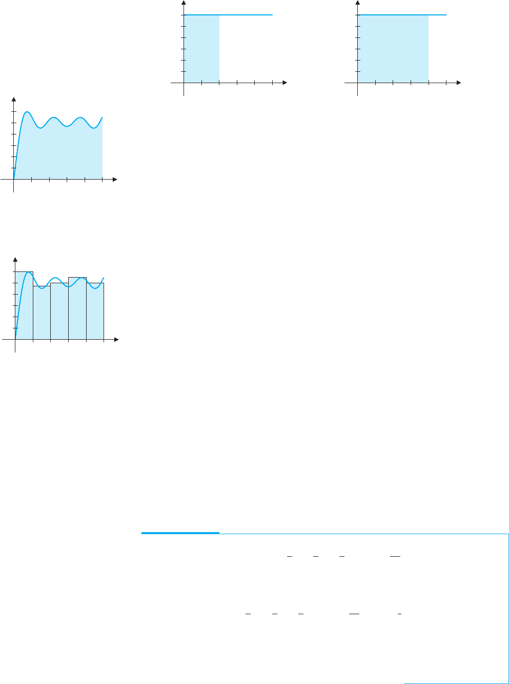
It’s no surprise that driving at a constant 60 mph, you travel 120 miles in 2 hours or 240
milesin 4hours.Viewingthis graphically,notethatthe areaunderthe graphofthe(constant)
velocity function v(t) = 60 from t = 0tot = 2 is 120, the distance traveled in this time in-
terval. (See the shaded area in Figure 4.2a on the following page.) Likewise, in Figure 4.2b,
the shaded region from t = 0tot = 4 has area equal to the distance of 240 miles.
P1: OSO/OVY P2: OSO/OVY QC: OSO/OVY T1: OSO
MHDQ256-Ch04 MHDQ256-Smith-v1.cls December 13, 2010 21:23
LT (Late Transcendental)
CONFIRMING PAGES
260 CHAPTER 4
..
Integration 4-10
Velocity
54321
Time
60
40
20
Velocity
54321
Time
60
40
20
FIGURE 4.2a
y = v(t) on [0, 2]
FIGURE 4.2b
y = v(t) on [0, 4]
It turns out that, in general, the distance traveled over a particular time interval equals
the area of the region bounded by y = v(t) and the t-axis on that interval. For the case of
constant velocity, this is no surprise, as we have that
d = r × t = velocity × time.
Our aim over the next several sections is to compute the area under the curve for a noncon-
stant function, such as the one shown in Figure 4.3. Our work in this section provides the
first step toward a powerful technique for computing such areas. To indicate the direction
we will take, note that we can approximate the area in Figure 4.3 by the sum of the areas of
the five rectangles indicated in Figure 4.4:
A ≈ 60 +45 +50 + 55 +50 = 260miles.
Of course, this is a crude estimate of the area, but you should observe that we could get a
better estimate by approximating the area using more (and smaller) rectangles. Certainly,
we had no problem adding up the areas of five rectangles, but for 5000 rectangles, you will
want some means for simplifying and automating the process. Dealing with such sums is
the topic of this section.
54321
60
40
20
x
y
FIGURE 4.3
Nonconstant velocity
y
54321
60
x
40
20
FIGURE 4.4
Approximate area
We begin by introducing some notation. Suppose that you want to sum the squares of
the first 20 positive integers. Notice that
1 + 4 + 9 +···+400 = 1
2
+ 2
2
+ 3
2
+···+20
2
,
where each term in the sum has the form i
2
, for i = 1, 2, 3,...,20. To reduce the amount
of writing, we use the Greek capital letter sigma,
, as a symbol for sum and write the sum
in summation notation as
20
i=1
i
2
= 1
2
+ 2
2
+ 3
2
+···+20
2
,
to indicate that we add together terms of the form i
2
, starting with i = 1 and ending with
i = 20. The variable i is called the index of summation.
In general, for any real numbers a
1
, a
2
,...,a
n
,wehave
n
i=1
a
i
= a
1
+ a
2
+···+a
n
.
EXAMPLE 2.1 Using Summation Notation
Write in summation notation: (a)
√
1 +
√
2 +
√
3 +···+
√
10 and
(b) 3
3
+ 4
3
+ 5
3
+···+45
3
.
Solution (a) We have the sum of the square roots of the integers from 1 to 10:
√
1 +
√
2 +
√
3 +···+
√
10 =
10
i=1
√
i.
(b) Similarly, the sum of the cubes of the integers from 3 to 45:
3
3
+ 4
3
+ 5
3
+···+45
3
=
45
i=3
i
3
.

P1: OSO/OVY P2: OSO/OVY QC: OSO/OVY T1: OSO
MHDQ256-Ch04 MHDQ256-Smith-v1.cls December 13, 2010 21:23
LT (Late Transcendental)
CONFIRMING PAGES
4-11 SECTION 4.2
..
Sums and Sigma Notation 261
EXAMPLE 2.2 Summation Notation for a Sum Involving Odd Integers
Write in summation notation: the sum of the first 200 odd positive integers.
Solution First, notice that (2i) is even for every integer i and hence, both (2i − 1) and
(2i +1) are odd. So, we have
1 + 3 + 5 +···+399 =
200
i=1
(2i −1).
Alternatively, we can write this as the equivalent expression
199
i=0
(2i +1). (Write out the
terms to see why these are equivalent.)
REMARK 2.1
The index of summation is a
dummy variable, since it is
used only as a counter to keep
track of terms. The value of the
summation does not depend on
the letter used as the index. For
this reason, you may use any
letter you like as an index. By
tradition, we most frequently
use i, j, k, m and n, but any
index will do. For instance,
n
i=1
a
i
=
n
j=1
a
j
=
n
k=1
a
k
.
EXAMPLE 2.3 Computing Sums Given in Summation Notation
Write out all terms and compute the sums (a)
8
i=1
(2i +1), (b)
6
i=2
sin(2πi) and (c)
10
i=4
5.
Solution (a) We have
8
i=1
(2i +1) = 3 + 5 + 7 + 9 + 11 + 13 + 15 + 17 = 80.
(b)
6
i=2
sin(2πi) = sin4π + sin 6π + sin8π +sin10π +sin 12π = 0.
(Note that the sum started at i = 2.) Finally, we have
(c)
10
i=4
5 = 5 + 5 + 5 + 5 + 5 +5 +5 = 35.
We give several shortcuts for computing sums in the following result.
THEOREM 2.1
If n is any positive integer and c is any constant, then
(i)
n
i=1
c = cn (sum of constants),
(ii)
n
i=1
i =
n(n +1)
2
(sum of the first n positive integers) and
(iii)
n
i=1
i
2
=
n(n +1)(2n +1)
6
(sum of the squares of the first n positive integers).
HISTORICAL
NOTES
Karl Friedrich Gauss
(1777–1855)
A German mathematician widely
considered to be the greatest
mathematician of all time. A
prodigy who had proved
important theorems by age 14,
Gauss was the acknowledged
master of almost all areas of
mathematics. He proved the
Fundamental Theorem of Algebra
and numerous results in number
theory and mathematical physics.
Gauss was instrumental in starting
new fields of research including
the analysis of complex variables,
statistics, vector calculus and
non-Euclidean geometry. Gauss
was truly the “Prince of
Mathematicians.’’
PROOF
(i)
n
i=1
c indicates to add the same constant c to itself n times and hence, the sum is simply
c times n.
(ii) The following clever proof has been credited to then 10-year-old Karl Friedrich Gauss.
(For more on Gauss, see the historical note in the margin.) First notice that
n
i=1
i = 1 + 2 + 3 +···+(n − 2) + (n − 1) + n
n terms
. (2.1)

P1: OSO/OVY P2: OSO/OVY QC: OSO/OVY T1: OSO
MHDQ256-Ch04 MHDQ256-Smith-v1.cls December 13, 2010 21:23
LT (Late Transcendental)
CONFIRMING PAGES
262 CHAPTER 4
..
Integration 4-12
Since the order in which we add the terms does not matter, we add the terms in (2.1) in
reverse order, to get
n
i=1
i = n + (n − 1) +(n − 2) +···+3 + 2 + 1
same n terms (backward)
. (2.2)
Adding equations (2.1) and (2.2) term by term, we get
2
n
i=1
i = (1 + n) + (2 + n − 1) + (3 + n − 2) +···+(n − 1 + 2) + (n + 1)
= (n + 1) +(n + 1) +(n + 1) +···+(n + 1) + (n + 1) +(n + 1)
n terms
= n(n + 1), Adding each term in parentheses.
since (n + 1) appears n times in the sum. Dividing both sides by 2 gives us
n
i=1
i =
n(n +1)
2
,
as desired. The proof of (iii) requires a more sophisticated proof using mathematical induc-
tion and we defer it to the end of this section.
We also have the following general rule for expanding sums. The proof is straight-
forward and is left as an exercise.
THEOREM 2.2
For any constants c and d,
n
i=1
(ca
i
+ db
i
) = c
n
i=1
a
i
+ d
n
i=1
b
i
.
Using Theorems 2.1 and 2.2, we can nowcompute severalsimple sums with ease. Note
that we have no more difficulty summing 800 terms than we do summing 8.
EXAMPLE 2.4 Computing Sums Using Theorems 2.1 and 2.2
Compute (a)
8
i=1
(2i +1) and (b)
800
i=1
(2i +1).
Solution (a) From Theorems 2.1 and 2.2, we have
8
i=1
(2i +1) = 2
8
i=1
i +
8
i=1
1 = 2
8(9)
2
+ (1)(8) = 72 +8 = 80.
(b) Similarly,
800
i=1
(2i +1) = 2
800
i=1
i +
800
i=1
1 = 2
800(801)
2
+ (1)(800)
= 640,800 +800 = 641,600.
EXAMPLE 2.5 Computing Sums Using Theorems 2.1 and 2.2
Compute (a)
20
i=1
i
2
and (b)
20
i=1
i
20
2
.
Solution (a) From Theorems 2.1 and 2.2, we have
20
i=1
i
2
=
20(21)(41)
6
= 2870.
(b)
20
i=1
i
20
2
=
1
20
2
20
i=1
i
2
=
1
400
20(21)(41)
6
=
1
400
2870 = 7.175.