Smith R., Minton R. Calculus
Подождите немного. Документ загружается.

P1: OSO/OVY P2: OSO/OVY QC: OSO/OVY T1: OSO
MHDQ256-Ch04 MHDQ256-Smith-v1.cls December 13, 2010 21:23
LT (Late Transcendental)
CONFIRMING PAGES
4-23 SECTION 4.4
..
The Definite Integral 273
4.4 THE DEFINITE INTEGRAL
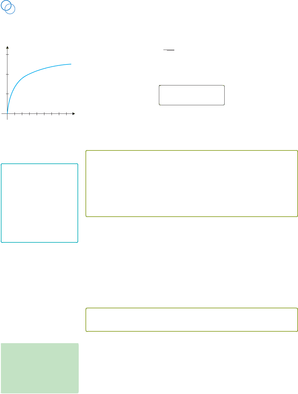
A sky diver who steps out of an airplane (starting with zero downward velocity) gradually
picks up speed until reaching terminal velocity, the speed at which the force due to air
resistance cancels out the force due to gravity. A function that models the velocity x seconds
into the jump is f (x) = 30
1 −
1
√
x+1
. (See Figure 4.12.)
We saw in section 4.2 that the area A under this curve on the interval 0 ≤ x ≤ t corre-
sponds to the distance fallen in the first t seconds. For any given value of t, the area is given
by the limit of the Riemann sums,
A = lim
n→∞
n
i=1
f (c
i
)x, (4.1)
where for each i, c
i
is taken to be any point in the subinterval [x
i−1
, x
i
].
Notice that the sum in (4.1) still makes sense even when some (or all) of the function
values f (c
i
) are negative. The general definition follows.
y
x
10
20
30
16
1412108642
FIGURE 4.12
y = f (x)
DEFINITION 4.1
For any function f defined on [a, b], the definite integral of f from a to b is
b
a
f (x) dx = lim
n→∞
n
i=1
f (c
i
)x,
whenever the limit exists and is the same for every choice of evaluation points,
c
1
, c
2
,...,c
n
. When the limit exists, we say that f is integrable on [a, b].
REMARK 4.1
Definition 4.1 is adequate for
most functions (those that are
continuous except for at
most a finite number of
discontinuities). For more
general functions, we broaden
the definition to include
partitions with subintervals of
different lengths. You can find a
suitably generalized definition
in Chapter 14.
Weshouldobservethatinthe Riemann sum,theGreek letter
indicatesa sum;sodoes
the elongated “S”,
used as the integralsign. The lower and upper limits of integration, a
andb,respectively, indicate the endpoints of the intervaloverwhich you are integrating.The
dx in the integral corresponds to the increment x in the Riemann sum and also indicates
the variable of integration. The letter used for the variable of integration (called a dummy
variable) is irrelevant since the value of the integral is a constant and not a function of x.
Here, f (x) is called the integrand.
So, when will the limit defining a definite integral exist? Theorem 4.1 indicates that
many familiar functions are integrable.
THEOREM 4.1
If f is continuous on the closed interval [a, b], then f is integrable on [a, b].
The proof of Theorem 4.1 is too technical to include here. However, if you think about
the area interpretation of the definite integral, the result should seem plausible.
NOTES
If f is continuous on [a, b] and
f (x) ≥ 0on[a, b], then
b
a
f (x)dx = Area under the
curve ≥ 0.
To calculate a definite integral of an integrable function, we have two options: if the
function is simple enough (say, a polynomial of degree 2 or less), we can symbolically
compute the limit of the Riemann sums. Otherwise, we can numerically compute a number
of Riemann sums and approximate the value of the limit. We frequently use the Midpoint
Rule, which uses the midpoints as the evaluation points for the Riemann sum.
P1: OSO/OVY P2: OSO/OVY QC: OSO/OVY T1: OSO
MHDQ256-Ch04 MHDQ256-Smith-v1.cls December 13, 2010 21:23
LT (Late Transcendental)
CONFIRMING PAGES
274 CHAPTER 4
..
Integration 4-24
EXAMPLE 4.1 A Midpoint Rule Approximation of a Definite Integral
Use the Midpoint Rule to estimate
15
0
30
1 −
1
√
x +1
dx.
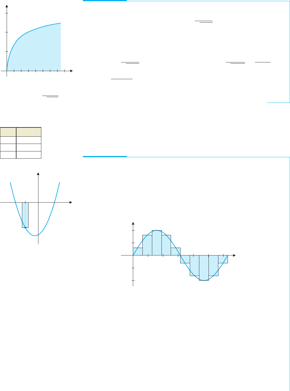
Solution The integral gives the area under the curve indicated in Figure 4.13. (Note
that this corresponds to the distance fallen by the sky diver in this section’s
introduction.) From the Midpoint Rule we have
15
0
30
1 −
1
√
x +1
dx ≈
n
i=1
f (c
i
)x = 30
n
i=1
1 −
1
√
c
i
+ 1
15 − 0
n
,
where c
i
=
x
i
+ x
i−1
2
. Using a CAS or a calculator program, you can get the sequence
of approximations found in the accompanying table.
One remaining question is when to stop increasing n. In this case, we continued to
increase n until it seemed clear that 270 feet was a reasonable approximation.
Now, think carefully about the limit in Definition 4.1. How can we interpret this limit
when f is both positive and negative on the interval [a, b]? Notice that if f (c
i
) < 0, for
some i, then the height of the rectangle shown in Figure 4.14 is −f (c
i
) and so,
f (c
i
)x =−Area of the ith rectangle.
To see the effect this has on the sum, consider example 4.2.
y
x
10
20
30
16
1412108642
10
20
42
FIGURE 4.13
y = 30
1 −
1
√
x + 1
n R
n
10 271.17
20 270.33
50 270.05
y
x
c
i
(c
i
, f (c
i
))
yf(x)
=
FIGURE 4.14
f (c
i
) < 0
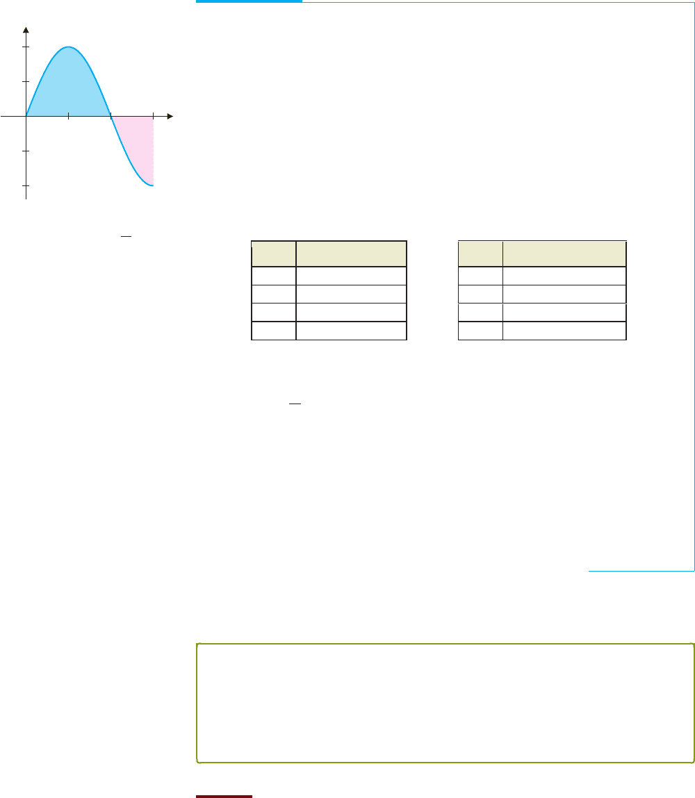
EXAMPLE 4.2 A Riemann Sum for a Function with Positive
and Negative Values
For f (x) = sin x on [0, 2π ], give an area interpretation of lim
n→∞
n
i=1
f (c
i
)x.
Solution For this illustration, we take c
i
to be the midpoint of [x
i−1
, x
i
], for
i = 1, 2,...,n. In Figure 4.15a, we see 10 rectangles constructed between the x-axis
and the curve y = f (x).
y
x
1.0
0.5
0.5
1.0
1
2 3
456
FIGURE 4.15a
Ten rectangles
The first five rectangles [where f (c
i
) > 0] lie above the x-axis and have height
f (c
i
). The remaining five rectangles [where f (c
i
) < 0] lie below the x-axis and have
height −f (c
i
). So, here
10
i=1
f (c
i
)x = (Area of rectangles above the x-axis)
−(Area of rectangles below the x-axis).
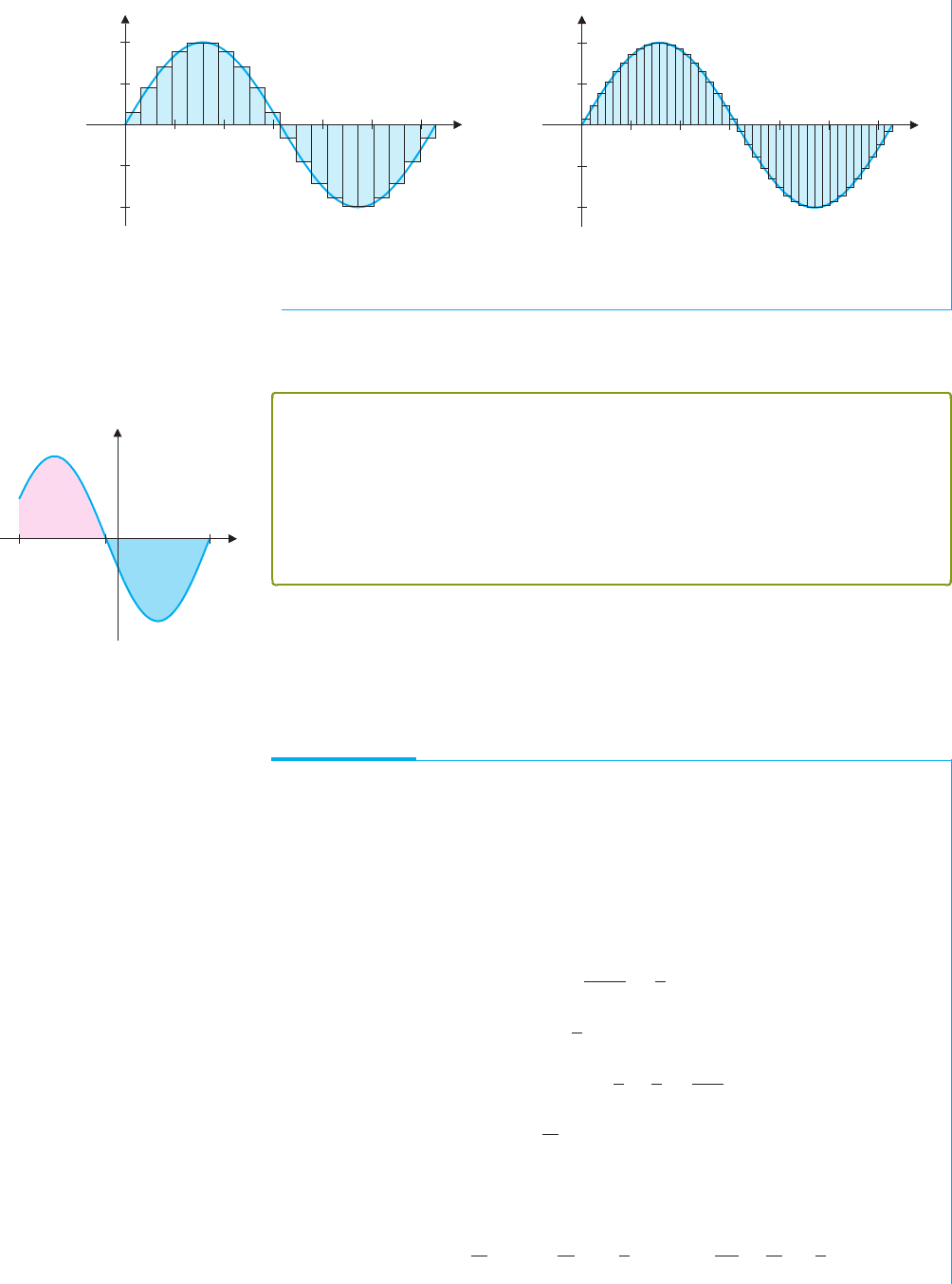
In Figures 4.15b and 4.15c, we show 20 and 40 rectangles, respectively, constructed in
the same way. From this, observe that
lim
n→∞
n
i=1
f (c
i
)x = (Area above the x-axis) −(Area below the x-axis),
which turns out to be zero, in this case.
P1: OSO/OVY P2: OSO/OVY QC: OSO/OVY T1: OSO
MHDQ256-Ch04 MHDQ256-Smith-v1.cls December 13, 2010 21:23
LT (Late Transcendental)
CONFIRMING PAGES
4-25 SECTION 4.4
..
The Definite Integral 275
x
−1.0
−0.5
0.5
1.0
1
2 3
456
y
1.0
1
2 3
456
x
y
1.0
0.5
0.5
FIGURE 4.15b
Twenty rectangles
FIGURE 4.15c
Forty rectangles
More generally, we have the notion of signed area, which we now define.
b
A
1
A
2
ac
y
x
FIGURE 4.16
Signed area
DEFINITION 4.2
Suppose that f (x) ≥ 0 on the interval [a, b] and A
1
is the area bounded between the
curve y = f (x) and the x-axis for a ≤ x ≤ b. Further, suppose that f (x) ≤ 0onthe
interval [b, c] and A
2
is the area bounded between the curve y = f (x) and the x-axis
for b ≤ x ≤ c. The signed area between y = f (x) and the x-axis for a ≤ x ≤ c is
A
1
− A
2
, and the total area between y = f (x) and the x-axis for a ≤ x ≤ c is
A
1
+ A
2
. (See Figure 4.16.)
Definition 4.2 says that signed area is the difference between any areas lying above the
x-axis and any areas lying below the x-axis, while the total area is the sum total of the area
bounded between the curve y = f (x) and the x-axis.
Example 4.3 examines the general case where the integrand may be both positive and
negative on the interval of integration.
EXAMPLE 4.3 Relating Definite Integrals to Signed Area
Compute the integrals: (a)
2
0
(x
2
− 2x)dx and (b)
3
0
(x
2
− 2x)dx, and interpret each in
terms of area.
Solution First, note that the integrand is continuous everywhere and so, it is also
integrable on any interval. (a) The definite integral is the limit of a sequence of Riemann
sums, where we can choose any evaluation points we wish. It is usually easiest to write
out the formula using right endpoints, as we do here. In this case,
x =
2 − 0
n
=
2
n
.
We then have x
0
= 0, x
1
= x
0
+ x =
2
n
,
x
2
= x
1
+ x =
2
n
+
2
n
=
2(2)
n
and so on. We then have c
i
= x
i
=
2i
n
. The nth Riemann sum R
n
is then
R
n
=
n
i=1
f (x
i
)x =
n
i=1
x
2
i
− 2x
i
x
=
n
i=1
2i
n
2
− 2
2i
n
2
n
=
n
i=1
4i
2
n
2
−
4i
n
2
n
P1: OSO/OVY P2: OSO/OVY QC: OSO/OVY T1: OSO
MHDQ256-Ch04 MHDQ256-Smith-v1.cls December 13, 2010 21:23
LT (Late Transcendental)
CONFIRMING PAGES
276 CHAPTER 4
..
Integration 4-26
=
8
n
3
n
i=1
i
2
−
8
n
2
n
i=1
i
=
8
n
3
n(n +1)(2n + 1)
6
−
8
n
2
n(n +1)
2
From Theorem 2.1 (ii) and (iii).
=
4(n + 1)(2n + 1)
3n
2
−
4(n + 1)
n
=
8n
2
+ 12n + 4
3n
2
−
4n + 4
n
.
Taking the limit of R
n
as n →∞gives us the exact value of the integral:
2
0
(x
2
− 2x)dx = lim
n→∞
8n
2
+ 12n + 4
3n
2
−
4n + 4
n
=
8
3
− 4 =−
4
3
.
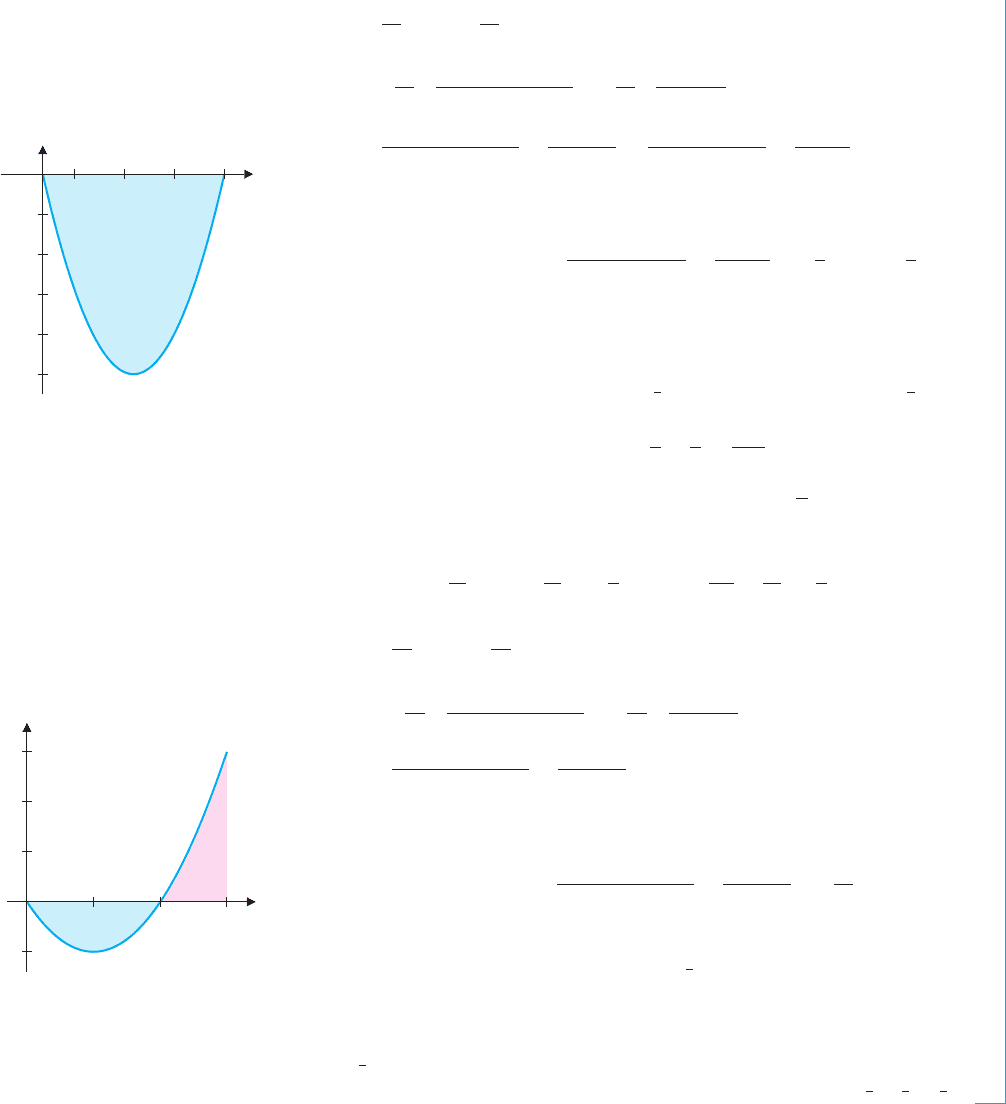
A graph of y = x
2
− 2x on the interval [0, 2] is shown in Figure 4.17. Notice that
since the function is always negative on the interval [0, 2], the integral is negative and
equals −A, where A is the area lying between the x-axis and the curve.
y
x
0.2
0.4
0.6
0.8
1.0
1.5
2.01.00.5
FIGURE 4.17
y = x
2
− 2x on [0, 2]
(b) On the interval [0, 3], we have x =
3
n
and x
0
= 0, x
1
= x
0
+ x =
3
n
,
x
2
= x
1
+ x =
3
n
+
3
n
=
3(2)
n
and so on. Using right-endpoint evaluation, we have c
i
= x
i
=
3i
n
. This gives us the
Riemann sum
R
n
=
n
i=1
3i
n
2
− 2
3i
n
3
n
=
n
i=1
9i
2
n
2
−
6i
n
3
n
=
27
n
3
n
i=1
i
2
−
18
n
2
n
i=1
i
=
27
n
3
n(n +1)(2n + 1)
6
−
18
n
2
n(n +1)
2
From Theorem 2.1 (ii) and (iii).
=
9(n + 1)(2n + 1)
2n
2
−
9(n + 1)
n
.
Taking the limit as n →∞gives us
3
0
(x
2
− 2x)dx = lim
n→∞
9(n + 1)(2n + 1)
2n
2
−
9(n + 1)
n
=
18
2
− 9 = 0.
On the interval [0, 2], notice that the curve y = x
2
− 2x lies below the x-axis and the
area bounded between the curve and the x-axis is
4
3
. On the interval [2, 3], the curve lies
above the x-axis and so, the integral of 0 on the interval [0, 3] indicates that the signed
areas have canceled out one another. (See Figure 4.18 for a graph of y = x
2
− 2x on the
interval [0, 3].) Note that this also says that the area under the curve on the interval [2, 3]
must be
4
3
. You should also observe that the total area A bounded between y = x
2
− 2x
and the x-axis is the sum of the two areas indicated in Figure 4.18, A =
4
3
+
4
3
=
8
3
.
y
x
3
2
1
1
1
2 3
FIGURE 4.18
y = x
2
− 2x on [0, 3]
We can also interpret signed area in terms of velocity and position. Suppose that v(t)is
thevelocityfunctionforanobjectmovingbackandforthalongastraightline. Noticethatthe
velocity may be both positive and negative. If the velocity is positive on the interval [t
1
, t
2
],
then
t
2
t
1
v(t)dt gives the distance traveled (here, in the positive direction). If the velocity
is negative on the interval [t
3
, t
4
], then the object is moving in the negative direction and
the distance traveled (here, in the negative direction) is given by −
t
4
t
3
v(t)dt. Notice that
if the object starts moving at time 0 and stops at time T, then
T
0
v(t)dt gives the distance
traveled in the positive direction minus the distance traveled in the negative direction. That
is,
T
0
v(t)dt corresponds to the overall change in position from start to finish.
P1: OSO/OVY P2: OSO/OVY QC: OSO/OVY T1: OSO
MHDQ256-Ch04 MHDQ256-Smith-v1.cls December 13, 2010 21:23
LT (Late Transcendental)
CONFIRMING PAGES
4-27 SECTION 4.4
..
The Definite Integral 277
EXAMPLE 4.4 Estimating Overall Change in Position
An object moving along a straight line has velocity function v(t) = sint. If the object
starts at position 0, determine the total distance traveled and the object’s position at time
t = 3π/2.
Solution From the graph (see Figure 4.19), notice that sint ≥ 0 for 0 ≤ t ≤ π and
sint ≤ 0 for π ≤ t ≤ 3π/2. The total distance traveled corresponds to the area of the
shaded regions in Figure 4.19, given by
A =
π
0
sintdt−
3π/2
π
sintdt.
You can use the Midpoint Rule to get the following Riemann sums:
y
t
0.5
0.5
1.0
1.0
3/2
/2
FIGURE 4.19
y = sin t on
0,
3π
2
n R
n
≈
π
0
sin tdt
10 2.0082
20 2.0020
50 2.0003
100 2.0001
n R
n
≈
3π/2
π
sin tdt
10 −1.0010
20 −1.0003
50 −1.0000
100 −1.0000
Observe that the sums appear to be converging to 2 and −1, respectively, which we will
soon be able to show are indeed correct. The total area bounded between y = sint and
the t-axis on
0,
3π
2
is then
π
0
sintdt−
3π/2
π
sintdt= 2 + 1 = 3,
so that the total distance traveled is 3 units. The overall change in position of the object
is given by
3π/2
0
sintdt=
π
0
sintdt+
3π/2
π
sintdt= 2 + (−1) = 1.
So, if the object starts at position 0, it ends up at position 0 + 1 = 1.
Next, we give some general rules for integrals.
THEOREM 4.2
If f and g are integrable on [a, b], then the following are true.
(i) For any constants c and d,
b
a
[cf(x) + dg(x)]dx = c
b
a
f (x) dx + d
b
a
g(x) dx
and
(ii) For any c in [a, b],
b
a
f (x) dx =
c
a
f (x) dx +
b
c
f (x) dx.
PROOF
By definition, for any constants c and d,wehave
b
a
[cf(x) + dg(x)]dx = lim
n→∞
n
i=1
[cf(c
i
) + dg(c
i
)]x
= lim
n→∞
c
n
i=1
f (c
i
)x + d
n
i=1
g(c
i
)x
From Theorem 2.2.
P1: OSO/OVY P2: OSO/OVY QC: OSO/OVY T1: OSO
MHDQ256-Ch04 MHDQ256-Smith-v1.cls December 13, 2010 21:23
LT (Late Transcendental)
CONFIRMING PAGES
278 CHAPTER 4
..
Integration 4-28
= c lim
n→∞
n
i=1
f (c
i
)x + d lim
n→∞
n
i=1
g(c
i
)x
= c
b
a
f (x) dx + d
b
a
g(x) dx,
where we have used our usual rules for summations plus the fact that f and g are integrable.
We leave the proof of part (ii) to the exercises, but note that we have already illustrated the
idea in example 4.4.
We now make a pair of reasonable definitions. First, for any integrable function f,if
a < b, we define
a
b
f (x) dx =−
b
a
f (x) dx. (4.2)
y
x
FIGURE 4.20
Piecewise continuous function
This should appear reasonable in that if we integrate “backward” along an interval, the
width of the rectangles corresponding to a Riemann sum (x) would seem to be negative.
Second, if f (a) is defined, we define
a
a
f (x) dx = 0.
If you think of the definite integral as area, this says that the area from a up to a is zero.
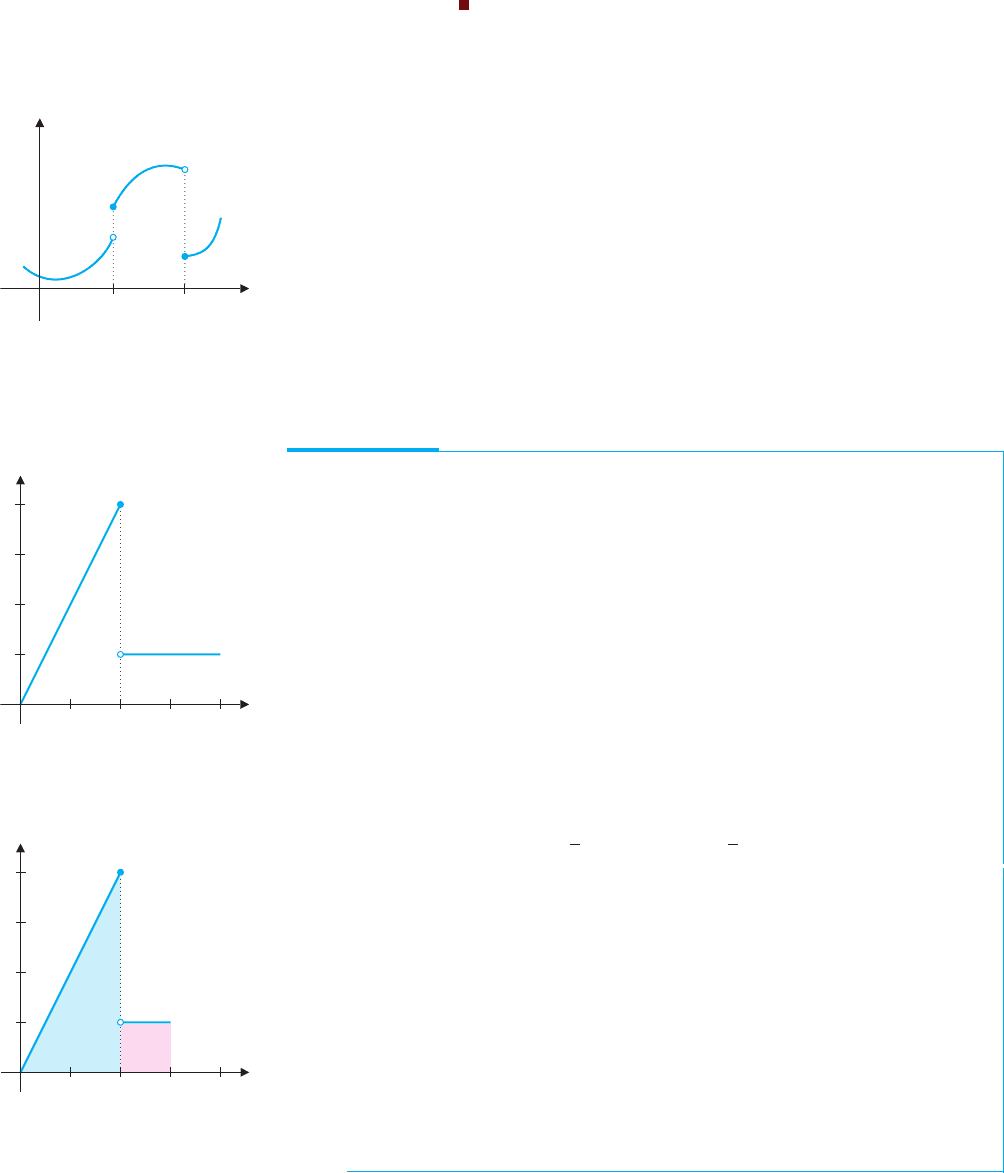
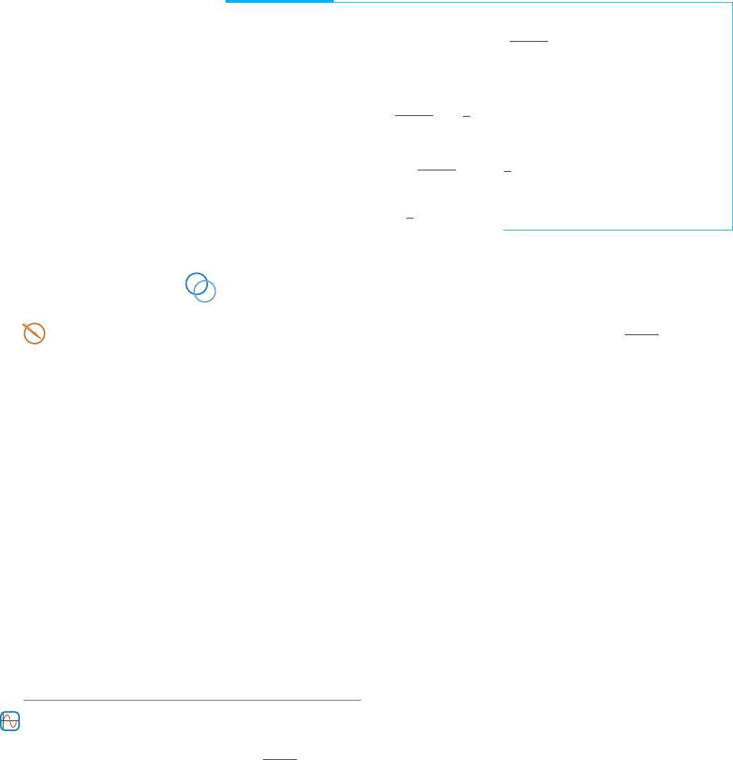
It turns out that a function is integrable even when it has a finite number of jump dis-
continuities, but is otherwise continuous. (Such a function is called piecewise continuous;
see Figure 4.20 for the graph of such a function.)
In example 4.5, we evaluate the integral of a discontinuous function.
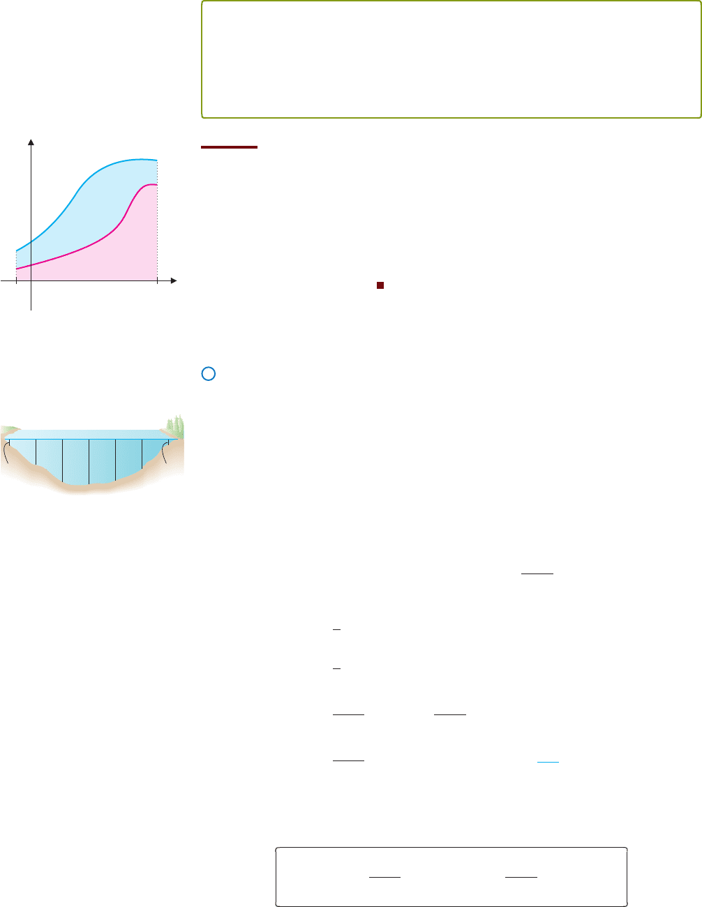
EXAMPLE 4.5 An Integral with a Discontinuous Integrand
Evaluate
3
0
f (x) dx, where f (x) is defined by
f (x) =
2x, if x ≤ 2
1, if x > 2
.
y
x
4
3
2
1
1
2 3 4
FIGURE 4.21a
y = f (x)
y
x
4
3
2
1
1
2 3 4
FIGURE 4.21b
The area under the curve y = f (x)
on [0, 3]
Solution We start by looking at a graph of y = f (x) in Figure 4.21a. Notice that
although f is discontinuous at x = 2, it has only a single jump discontinuity and so, is
piecewise continuous on [0, 3]. By Theorem 4.2 (ii), we have that
3
0
f (x) dx =
2
0
f (x) dx +
3
2
f (x) dx.
Referring to Figure 4.21b, observe that
2
0
f (x) dx corresponds to the area of the
triangle of base 2 and altitude 4 shaded in the figure, so that
2
0
f (x) dx =
1
2
(base) (height) =
1
2
(2)(4) = 4.
Next, also notice from Figure 4.21b that
3
2
f (x) dx corresponds to the area of the
square of side 1, so that
3
2
f (x) dx = 1.
We now have that
3
0
f (x) dx =
2
0
f (x) dx +
3
2
f (x) dx = 4 + 1 = 5.
Notice that in this case, the areas corresponding to the two integrals could be computed
using simple geometric formulas and so, there was no need to compute Riemann sums
here.
P1: OSO/OVY P2: OSO/OVY QC: OSO/OVY T1: OSO
MHDQ256-Ch04 MHDQ256-Smith-v1.cls December 13, 2010 21:23
LT (Late Transcendental)
CONFIRMING PAGES
4-29 SECTION 4.4
..
The Definite Integral 279
Another simple property of definite integrals is the following.
THEOREM 4.3
Suppose that g(x) ≤ f (x) for all x ∈ [a, b] and that f and g are integrable on [a, b].
Then,
b
a
g(x) dx ≤
b
a
f (x) dx.
PROOF
Since g(x) ≤ f (x), we must also have that 0 ≤ [ f (x) − g(x)] on [a, b] and in view of this,
b
a
[ f (x) − g(x)]dx represents the area under the curve y = f (x) − g(x), which can’t be
negative. Using Theorem 4.2 (i), we now have
0 ≤
b
a
[ f (x) − g(x)]dx =
b
a
f (x) dx −
b
a
g(x) dx,
from which the result follows.
y = g(x)
y = ƒ(x)
x
y
ba
FIGURE 4.22
Larger functions have larger
integrals
Notice that Theorem 4.3 simply says that larger functions have larger integrals. We
illustrate this for the case of two positive functions in Figure 4.22.
x
0
x
1
x
2
x
n
f (x
0
) f (x
n
)
. . .
FIGURE 4.23
Average depth of a cross section
of a lake
Average Value of a Function
To compute the average age of the students in your calculus class, note that you need only
add up each student’s age and divide the total by the number of students in your class. By
contrast, how would you find the average depth of a cross section of a lake? You would get
a reasonable idea of the average depth by sampling the depth of the lake at a number of
points spread out along the length of the lake and then averaging these depths, as indicated
in Figure 4.23.
More generally, we often want to calculate the average value of a function f on some
interval [a, b]. To do this, we form a partition of [a, b]:
a = x
0
< x
1
< ···< x
n
= b,
where the difference between successive points is x =
b −a
n
. The average value, f
ave
,
is then given approximately by the average of the function values at x
1
, x
2
,...,x
n
:
f
ave
≈
1
n
[ f (x
1
) + f (x
2
) +···+ f (x
n
)]
=
1
n
n
i=1
f (x
i
)
=
1
b −a
n
i=1
f (x
i
)
b −a
n
Multiply and divide by (b −a).
=
1
b −a
n
i=1
f (x
i
)x. Since x =
b −a
n
.
Notice that the last summation is a Riemann sum. Further, observe that the more points we
sample, the better our approximation should be. So, lettingn →∞, we arrive at an integral
representing average value:
f
ave
= lim
n→∞
1
b −a
n
i=1
f (x
i
)x
=
1
b −a
b
a
f (x) dx. (4.3)
P1: OSO/OVY P2: OSO/OVY QC: OSO/OVY T1: OSO
MHDQ256-Ch04 MHDQ256-Smith-v1.cls December 13, 2010 21:23
LT (Late Transcendental)
CONFIRMING PAGES
280 CHAPTER 4
..
Integration 4-30
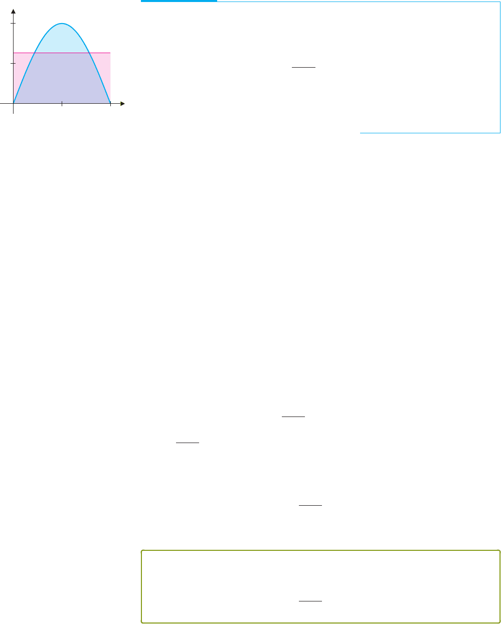
EXAMPLE 4.6 Computing the Average Value of a Function
Compute the average value of f (x) = sin x on the interval [0,π].
Solution From (4.3), we have
f
ave
=
1
π −0
π
0
sin xdx.
We can approximate the value of this integral by calculating some Riemann sums, to
obtain the approximate average, f
ave
≈ 0.6366198. (See example 4.4.) In Figure 4.24,
we show a graph of y = sin x and its average value on the interval [0,π]. You should
note that the two shaded regions have the same area.
y
x
0.5
1.0
p
q
f
ave
FIGURE 4.24
y = sin x and its average
Notice in Figure 4.24 that there are two points at which the function equals its average
value.Wegiveaprecisestatement ofthis(unsurprising)resultin Theorem4.4.First,observe
that for any constant, c,
b
a
cdx= lim
n→∞
n
i=1
c x = c lim
n→∞
n
i=1
x = c(b −a),
since
n
i=1
x is simply the sum of the lengths of the subintervals in the partition.
Let f be any continuous function defined on [a, b]. Recall that by the Extreme Value
Theorem, since f is continuous, it has a minimum, m, and a maximum, M,on[a, b], so that
m ≤ f (x) ≤ M, for all x ∈ [a, b]
and consequently, from Theorem 4.3,
b
a
mdx≤
b
a
f (x) dx ≤
b
a
Mdx.
Since m and M are constants, we get
m(b − a) ≤
b
a
f (x) dx ≤ M(b − a). (4.4)
Finally, dividing by (b −a) > 0, we obtain
m ≤
1
b −a
b
a
f (x) dx ≤ M.
That is,
1
b −a
b
a
f (x) dx (the average value of f on [a, b]) lies between the minimum
and the maximum values of f on [a, b]. Since f is a continuous function, we have by the
IntermediateValueTheorem(Theorem 4.4 in section 1.4) thattheremustbe some c ∈ (a, b)
for which
f (c) =
1
b −a
b
a
f (x) dx.
We have just proved a theorem:
THEOREM 4.4 (Integral Mean Value Theorem)
If f is continuous on [a, b], then there is a number c ∈ (a, b) for which
f (c) =
1
b −a
b
a
f (x) dx.
The Integral Mean Value Theorem is a fairly simple idea (that a continuous function
will take on its average value at some point), but it has some significant applications. The
first of these will be found in section 4.5, in the proof of one of the most significant results
in the calculus, the Fundamental Theorem of Calculus.
P1: OSO/OVY P2: OSO/OVY QC: OSO/OVY T1: OSO
MHDQ256-Ch04 MHDQ256-Smith-v1.cls December 13, 2010 21:23
LT (Late Transcendental)
CONFIRMING PAGES
4-31 SECTION 4.4
..
The Definite Integral 281
ReferringbacktoourderivationoftheIntegralMeanValueTheorem,observethatalong
the way we proved that for any integrable function f,ifm ≤ f (x) ≤ M, for all x ∈ [a, b],
then inequality (4.4) holds:
m(b − a) ≤
b
a
f (x) dx ≤ M(b − a).
Thisenables us to estimate the valueofadefiniteintegral.Althoughtheestimateisgenerally
only a rough one, it still has importance in that it gives us an interval in which the value
must lie. We illustrate this in example 4.7.
EXAMPLE 4.7 Estimating the Value of an Integral
Use inequality (4.4) to estimate the value of
1
0
x
2
+ 1 dx.
Solution First, notice that it’s beyond your present abilities to compute the value of
this integral exactly. However, notice that
1 ≤
x
2
+ 1 ≤
√
2, for all x ∈ [0, 1].
From inequality (4.4), we now have
1 ≤
1
0
x
2
+ 1 dx ≤
√
2 ≈ 1.414214.
In other words, although we still do not know the exact value of the integral, we know
that it must be between 1 and
√
2 ≈ 1.414214.
EXERCISES 4.4
WRITING EXERCISES
1. Sketch a graph of a function f that has both positive and neg-
ative values on an interval[a, b]. Explain in terms of area what
it means to have
b
a
f (x) dx = 0. Also, explain what it means
to have
b
a
f (x) dx > 0 and
b
a
f (x) dx < 0.
2. To get a physical interpretation of the result in Theorem 4.3,
suppose that f (x) and g(x) are velocity functions for two dif-
ferentobjects startingatthesameposition.If f (x) ≥ g(x) ≥ 0,
explain why it follows that
b
a
f (x) dx ≥
b
a
g(x)dx.
3. The Integral Mean Value Theorem says that if f (x) is continu-
ous on the interval [a, b], then thereexists a number c between
a and b such that f (c)(b − a) =
b
a
f (x) dx. By thinking of
the left-hand side of this equation as the area of a rectangle,
sketch a picture that illustrates this result, and explain why the
result follows.
4. Write out the Integral Mean Value Theorem as applied to the
derivative f
(x). Then write out the Mean Value Theorem for
derivatives. (See section 2.8.) If the c-values identified byeach
theorem are the same, what does
b
a
f
(x)dx have to equal?
Explain why, at this point, we don’t know whether or not the
c-values are the same.
In exercises 1–4, use the Midpoint Rule with n 6 to estimate
the value of the integral.
1.
3
0
(x
3
+ x)dx 2.
3
0
x
2
+ 1dx
3.
π
0
sin x
2
dx 4.
2
−2
4 − x
2
dx
............................................................
In exercises 5–8, give an area interpretation of the integral.
5.
3
1
x
2
dx 6.
1
0
(x
3
+ 1)dx
7.
2
0
(x
2
− 2)dx 8.
2
0
(x
3
− 3x
2
+ 2x)dx
............................................................
In exercises 9–14, evaluate the integral by computing the limit
of Riemann sums.
9.
1
0
2xdx 10.
2
1
2xdx
11.
2
0
x
2
dx 12.
3
0
(x
2
+ 1)dx
13.
3
1
(x
2
− 3)dx 14.
2
−2
(x
2
− 1)dx
............................................................
In exercises 15–20, write the given (total) area as an integral or
sum of integrals.
15. The area above the x-axis and below y = 4 − x
2
16. The area above the x-axis and below y = 4x − x
2
P1: OSO/OVY P2: OSO/OVY QC: OSO/OVY T1: OSO
MHDQ256-Ch04 MHDQ256-Smith-v1.cls December 13, 2010 21:23
LT (Late Transcendental)
CONFIRMING PAGES
282 CHAPTER 4
..
Integration 4-32
17. The area below the x-axis and above y = x
2
− 4
18. The area below the x-axis and above y = x
2
− 4x
19. The area between y = sin x and the x-axis for 0 ≤ x ≤ π
20. The area between y = sin x and the x-axis for
−
π
2
≤ x ≤
π
4
.
............................................................
In exercises 21 and 22, use the given velocity function and initial
position to estimate the final position s(b).
21. v(t) =
1
√
t
2
+ 1
, s(0) = 0, b = 4
22. v(t) =
30
√
t + 1
, s(0) =−1, b = 4
............................................................
In exercises 23 and 24, compute
4
0
f (x) dx.
23. f (x) =
2x if x < 1
4ifx ≥ 1
24. f (x) =
2ifx ≤ 2
3x if x > 2
............................................................
In exercises 25–28, compute the average value of the function
on the given interval.
25. f (x) = 2x + 1, [0, 4] 26. f (x) = x
2
+ 2x, [0, 1]
27. f (x) = x
2
− 1, [1, 3] 28. f (x) = 2x − 2x
2
, [0, 1]
............................................................
In exercises 29–32, use the Integral Mean Value Theorem to
estimate the value of the integral.
29.
π/2
π/3
3cos x
2
dx 30.
1/2
0
1
√
1 − x
2
dx
31.
2
0
2x
2
+ 1dx 32.
1
−1
3
x
3
+ 2
dx
............................................................
In exercises 33 and 34, find a value of c that satisfies the conclu-
sion of the Integral Mean Value Theorem.
33.
2
0
3x
2
dx (= 8) 34.
1
−1
(x
2
− 2x)dx (=
2
3
)
............................................................
In exercises 35 and 36, use Theorem 4.2 to write the expression
as a single integral.
35. (a)
2
0
f (x) dx +
3
2
f (x) dx (b)
3
0
f (x) dx −
3
2
f (x) dx
36. (a)
2
0
f (x) dx +
1
2
f (x) dx (b)
2
−1
f (x) dx +
3
2
f (x) dx
............................................................
In exercises 37 and 38, assume that
3
1
f (x) dx 3 and
3
1
g(x) dx −2 and find
37. (a)
3
1
[ f (x) + g(x)] dx (b)
3
1
[2 f (x) − g(x)] dx
38. (a)
3
1
[ f (x) − g(x)] dx (b)
3
1
[4g(x) −3 f (x)]dx
............................................................
In exercises 39 and 40, sketch the area corresponding to the
integral.
39. (a)
2
1
(x
2
− x)dx (b)
4
2
(x
2
− x)dx
40. (a)
π/2
0
cos xdx (b)
2
−2
4 − x
2
dx
............................................................
41. (a) Use Theorem 4.3 to showthat sin (1) ≤
2
1
x
2
sin xdx≤ 4.
(b) UseTheorem4.3toshowthat
7
3
sin1 ≤
2
1
x
2
sin xdx ≤
7
3
.
(c) Is the result of part (b) more useful than that of part (a)?
Briefly explain.
42. Use Theorem 4.3 to find bounds for
2
1
x
2
cos
√
xdx.
43. Prove that if f is continuous on the interval [a, b], then there
exists a number c in (a, b) such that f (c) equals the average
value of f on the interval [a, b].
44. Prove part (ii) of Theorem 4.2 for the special case where
c =
1
2
(a + b).
............................................................
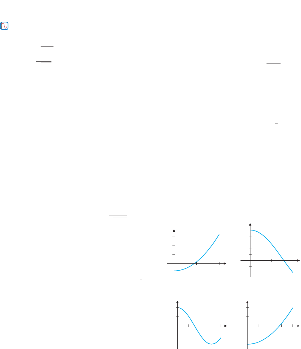
In exercises 45–48, use the graph to determine whether
2
0
f (x) dx is positive or negative.
45.
46.
x
y
21
3
2
1
1
x
y
2.01.51.00.5
1.0
0.8
0.6
0.4
0.2
0.2
0.4
47.
48.
x
y
2.01.51.00.5
1.0
0.5
0.5
1.0
x
y
2.01.51.00.5
2
1
1
2
............................................................