Smith R., Minton R. Calculus
Подождите немного. Документ загружается.

P1: OSO/OVY P2: OSO/OVY QC: OSO/OVY T1: OSO
MHDQ256-Ch04 MHDQ256-Smith-v1.cls December 13, 2010 21:23
LT (Late Transcendental)
CONFIRMING PAGES
4-13 SECTION 4.2
..
Sums and Sigma Notation 263
In the beginning of this section, we approximated distance by summing several values
of the velocity function. In section 4.3, we will further develop these sums to allow us to
compute areas exactly. However, our immediate interest in sums is to use these to sum a
number of values of a function, as we illustrate in examples 2.6 and 2.7.
EXAMPLE 2.6 Computing a Sum of Function Values
Sum the values of f (x) = x
2
+ 3 evaluated at x = 0.1, x = 0.2,...,x = 1.0.
Solution We first formulate this in summation notation, so that we can
use the rules we have developed in this section. The terms to be summed are
a
1
= f (0.1) = 0.1
2
+ 3, a
2
= f (0.2) = 0.2
2
+ 3 and so on. Note that since each of the
x-values is a multiple of 0.1, we can write the x’s in the form 0.1i, for i = 1, 2,...,10.
In general, we have
a
i
= f (0.1i) = (0.1i)
2
+ 3, for i = 1, 2,...,10.
From Theorem 2.1 (i) and (iii), we then have
10
i=1
a
i
=
10
i=1
f (0.1i) =
10
i=1
[(0.1i)
2
+ 3] = 0.1
2
10
i=1
i
2
+
10
i=1
3
= 0.01
10(11)(21)
6
+ (3)(10) = 3.85 +30 = 33.85.
EXAMPLE 2.7 A Sum of Function Values at Equally Spaced x’s
Sum the values of f (x) = 3x
2
− 4x + 2 evaluated at x = 1.05, x = 1.15,
x = 1.25,...,x = 2.95.
Solution You will need to think carefully about the x’s. The distance between
successive x-values is 0.1 and there are 20 such values. (Be sure to count these for
yourself.) Notice that we can write the x’s in the form 0.95 +0.1i, for i = 1, 2,...,20.
We now have
20
i=1
f (0.95 +0.1i) =
20
i=1
[3(0.95 + 0.1i)
2
− 4(0.95 +0.1i) + 2]
=
20
i=1
(0.03i
2
+ 0.17i + 0.9075) Multiply out terms.
= 0.03
20
i=1
i
2
+ 0.17
20
i=1
i +
20
i=1
0.9075 From Theorem 2.2.
= 0.03
20(21)(41)
6
+ 0.17
20(21)
2
+ 0.9075(20)
From Theorem 2.1
(i), (ii) and (iii).
= 139.95.
Over the next several sections, we will see how sums such as those found in examples
2.6 and 2.7 play a very significant role. We end this section by looking at a powerful
mathematical principle.
Principle of Mathematical Induction
For any proposition that depends on a positive integer, n, we first show that the result is
true for a specific value n = n
0
. We then assume that the result is true for an unspecified
n = k ≥ n
0
. (This is called the induction assumption.) If we can show that it follows that
the proposition is true for n = k + 1, then we have proved that the result is true for any

P1: OSO/OVY P2: OSO/OVY QC: OSO/OVY T1: OSO
MHDQ256-Ch04 MHDQ256-Smith-v1.cls December 13, 2010 21:23
LT (Late Transcendental)
CONFIRMING PAGES
264 CHAPTER 4
..
Integration 4-14
positive integer n ≥ n
0
. Think about why this must be true. (Hint: If P
1
is true and P
k
true
implies P
k+1
istrue,then P
1
trueimplies P
2
istrue,whichinturnimplies P
3
istrueandsoon.)
We can now use mathematical induction to prove the last part of Theorem 2.1, which
states that for any positive integer n,
n
i=1
i
2
=
n(n +1)(2n + 1)
6
.
PROOF OF THEOREM 2.1 (iii)
For n = 1, we have
1 =
1
i=1
i
2
=
1(2)(3)
6
,
as desired. So, the proposition is true for n = 1. Next, assume that
k
i=1
i
2
=
k(k + 1)(2k + 1)
6
,
Induction assumption. (2.3)
for some integer k ≥ 1.
In this case, we have by the induction assumption that for n = k + 1,
n
i=1
i
2
=
k+1
i=1
i
2
=
k
i=1
i
2
+
k+1
i=k+1
i
2
Split off the last term.
=
k(k + 1)(2k + 1)
6
+ (k + 1)
2
From (2.3).
=
k(k + 1)(2k + 1) +6(k + 1)
2
6
Add the fractions.
=
(k + 1)[k(2k + 1) + 6(k + 1)]
6
Factor out (k + 1).
=
(k + 1)[2k
2
+ 7k + 6]
6
Combine terms.
=
(k + 1)(k + 2)(2k + 3)
6
Factor the quadratic.
=
(k + 1)[(k + 1) + 1][2(k +1) +1]
6
Rewrite the terms.
=
n(n +1)(2n + 1)
6
,
Since n = k + 1.
as desired.
EXERCISES 4.2
WRITING EXERCISES
1. In the text, we mentioned that one of the benefits of using
the summation notation is the simplification of calculations.
To help understand this, write out in words what is meant by
40
i=1
(2i
2
− 4i + 11).
2. Following up on exercise 1, calculate the sum
40
i=1
(2i
2
− 4i +
11) and then describe in words how you did so. Be sure to
describe any formulas and your use of them in words.
In exercises 1 and 2, translate into summation notation.
1. 2(1)
2
+ 2(2)
2
+ 2(3)
2
+···+2(14)
2
2.
√
2 − 1 +
√
3 − 1 +
√
4 − 1 +···+
√
15 − 1
............................................................
In exercises 3 and 4, calculations are described in words.
Translate each into summation notation and then compute
the sum.
3. (a) The sum of the squares of the first 50 positive integers.
(b) The square of the sum of the first 50 positive integers.
P1: OSO/OVY P2: OSO/OVY QC: OSO/OVY T1: OSO
MHDQ256-Ch04 MHDQ256-Smith-v1.cls December 13, 2010 21:23
LT (Late Transcendental)
CONFIRMING PAGES
4-15 SECTION 4.2
..
Sums and Sigma Notation 265
4. (a) The sum of the square roots of the first 10 positive integers.
(b) The square root of the sum of the first 10 positive integers.
............................................................
In exercises 5–8, write out all terms and compute the sums.
5.
6
i=1
3i
2
6.
7
i=3
(i
2
+i)
7.
10
i=6
(4i + 2) 8.
8
i=6
(i
2
+ 2)
............................................................
In exercises 9–18, use summation rules to compute the sum.
9.
70
i=1
(3i − 1) 10.
45
i=1
(3i − 4)
11.
40
i=1
4 −i
2
12.
50
i=1
(8 −i)
13.
100
n=1
n
2
− 3n + 2
14.
140
n=1
n
2
+ 2n − 4
15.
30
i=3
[(i − 3)
2
+ (i − 3)] 16.
20
i=4
[(i − 3)(i + 3)]
17.
n
k=3
(k
2
− 3) 18.
n
k=0
(k
2
+ 5)
............................................................
In exercises 19–22, compute sums of the form
n
i1
f (x
i
)x for
the given values of x
i
.
19. f (x) = x
2
+ 4x; x = 0.2, 0.4, 0.6, 0.8, 1.0; x = 0.2; n = 5
20. f (x) = 3x + 5; x = 0.4, 0.8, 1.2, 1.6, 2.0; x = 0.4; n = 5
21. f (x) = 4x
2
− 2; x = 2.1, 2.2, 2.3, 2.4,...,3.0;
x = 0.1; n = 10
22. f (x) = x
3
+ 4; x = 2.05, 2.15, 2.25, 2.35,...,2.95;
x = 0.1; n = 10
............................................................
In exercises 23–26, compute the sum and the limit of the sum
as n → ∞.
23.
n
i=1
1
n
i
n
2
+ 2
i
n
24.
n
i=1
1
n
i
n
2
− 5
i
n
25.
n
i=1
1
n
4
2i
n
2
−
2i
n
26.
n
i=1
1
n
2i
n
2
+ 4
i
n
............................................................
27. Use mathematical induction to prove that
n
i=1
i
3
=
n
2
(n + 1)
2
4
for all integers n ≥ 1.
28. Use mathematical induction to prove that
n
i=1
i
5
=
n
2
(n + 1)
2
(2n
2
+ 2n − 1)
12
for all integers n ≥ 1.
............................................................
In exercises 29–32, use the formulas in exercises 27 and 28 to
compute the sums.
29.
10
i=1
(i
3
− 3i + 1) 30.
20
i=1
(i
3
+ 2i)
31.
100
i=1
(i
5
− 2i
2
) 32.
100
i=1
(2i
5
+ 2i + 1)
............................................................
33. Prove Theorem 2.2.
34. Use induction to derive the geometric series formula
a + ar +ar
2
+···+ar
n
=
a − ar
n+1
1 −r
for constants a and
r = 1.
............................................................
In exercises 35 and 36, use the result of exercise 34 to evaluate
the sum and the limit of the sum as n → ∞.
35.
n
i=1
3
1
4
i
36.
n
i=1
2
−1
3
i
APPLICATIONS
37. Suppose that a car has velocity 50 mph for 2 hours, velocity
60mph for 1 hour,velocity 70 mph for 30 minutes and velocity
60 mph for 3 hours. Find the distance traveled.
38. Suppose that a car has velocity 50 mph for 1 hour, velocity
40mph for 1 hour,velocity 60 mph for 30 minutes and velocity
55 mph for 3 hours. Find the distance traveled.
39. The table shows the velocity of a projectile at various times.
Estimate the distance traveled.
time (s) 0 0.25 0.5 0.75 1.0 1.25 1.5 1.75 2.0
velocity (ft/s) 120 116 113 110 108 106 104 103 102
40. The table shows the (downward) velocity of a falling object.
Estimate the distance fallen.
time (s) 0 0.5 1.0 1.5 2.0 2.5 3.0 3.5 4.0
velocity (m/s) 10 14.9 19.8 24.7 29.6 34.5 39.4 44.3 49.2
EXPLORATORY EXERCISES
1. Suppose that the velocity of a car is given by v(t) = 3
√
t +
30 mph at time t hours (0 ≤ t ≤ 4). We will try to deter-
mine the distance traveled in the 4 hours. The velocity at
t = 0isv(0) = 3
√
0 + 30 = 30 mph and the velocity at
time t = 1isv(1) = 3
√
1 + 30 = 33 mph. Since the aver-
age of these velocities is 31.5 mph, we could estimate that
the car traveled 31.5 miles in the first hour. Carefully explain
why this is not necessarily correct. Since v(1) = 33 mph and
v(2) = 3
√
2 + 30 ≈ 34 mph, we estimate that the car traveled
33.5 miles in the second hour. Using v(3) ≈ 35 mph and
v(4) = 36 mph, find similar estimates for the distance traveled
in the third and fourth hours and then estimate the total dis-
tance. To improvethis estimate, we can find an estimate for the
distance covered each half hour. The first estimate would take
v(0) = 30 mph and v(0.5) ≈ 32.1 mph and estimate a distance
of 15.525 miles. Estimate the average velocity and then the
distance for the remaining 7 half hours and estimate the total
distance. By estimating the average velocity every quarter
hour, find a third estimate of the total distance. Based on these
P1: OSO/OVY P2: OSO/OVY QC: OSO/OVY T1: OSO
MHDQ256-Ch04 MHDQ256-Smith-v1.cls December 13, 2010 21:23
LT (Late Transcendental)
CONFIRMING PAGES
266 CHAPTER 4
..
Integration 4-16
three estimates, conjecture the limit of these approximations
as the time interval considered goes to zero.
2. In this exercise, we investigate a generalization of a finite sum
called an infinite series. Suppose a bouncing ball has coeffi-
cient of restitution equal to 0.6. This means that if the ball hits
the ground with velocity v ft/s, it rebounds with velocity 0.6v.
Ignoring air resistance, a ball launchedwith velocity v ft/s will
stay in the air v/16 seconds before hitting the ground. Suppose
a ball with coefficient of restitution 0.6 is launched with initial
velocity 60 ft/s. Explain why the total time in the air is given
by 60/16 + (0.6)(60)/16 +(0.6)(0.6)(60)/16 +···. It might
seem like the ball would continue to bounce forever. To see
otherwise, use the result of exercise 34 to find the limit that
these sums approach. The limit is the number of seconds that
the ball continues to bounce.
3. The following statement is obviously false: Given any set
of n numbers, the numbers are all equal. Find the flaw in
the attempted use of mathematical induction. Let n = 1. One
numberisequalto itself. Assume thatforn = k,anyk numbers
are equal. Let S be any set of k + 1 numbers a
1
, a
2
,...,a
k+1
.
By the induction hypothesis, the first k numbers are equal:
a
1
= a
2
=···=a
k
and the last k numbers are equal:
a
2
= a
3
=···=a
k+1
.Combining theseresults,allk + 1 num-
bers are equal: a
1
= a
2
=···=a
k
= a
k+1
, as desired.
4.3 AREA
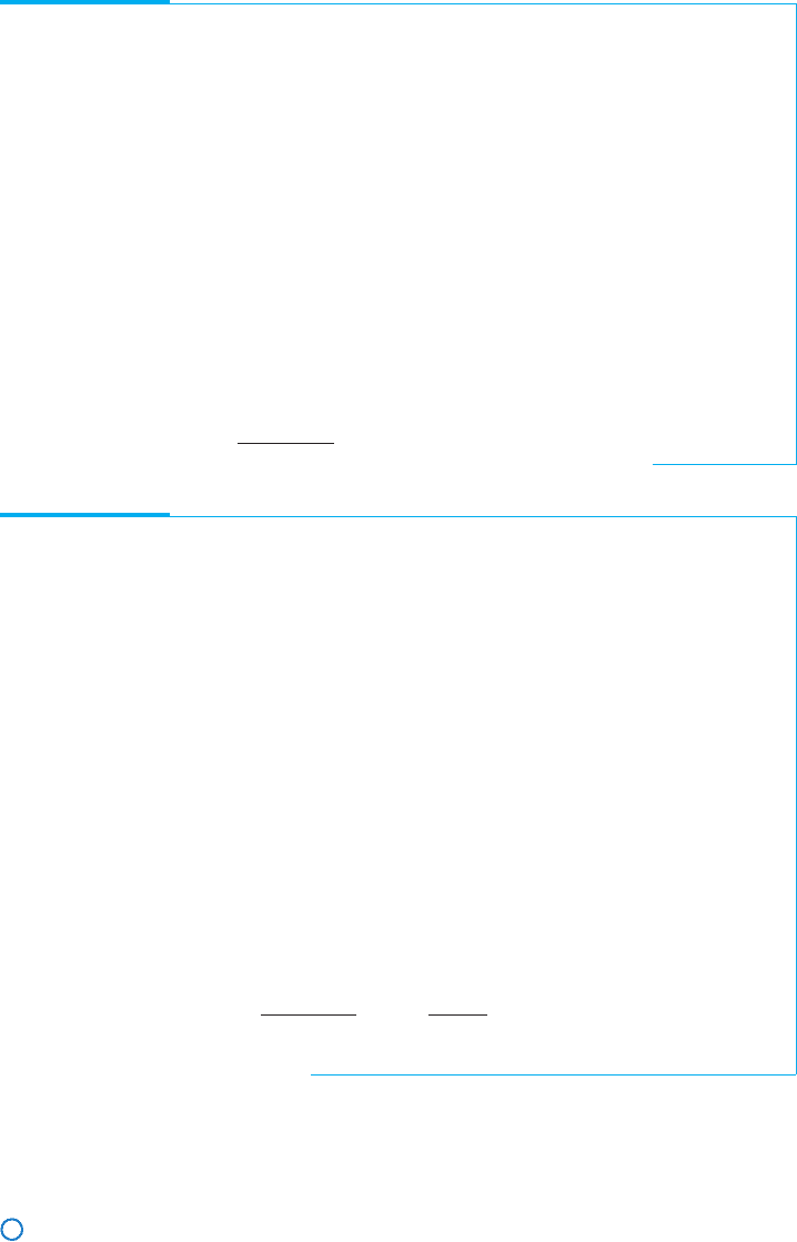
In this section, we develop a method for computing the area beneath the graph of y = f (x)
and above the x-axis on an interval a ≤ x ≤ b. You are familiar with the formulas for
computing the area of a rectangle, a circle and a triangle. However, howwould you compute
the area of a region that’s not a rectangle, circle or triangle?
We need a more general description of area, one that can be used to find the area of
almost any two-dimensional region imaginable. It turns out that this process (which we
generalize to the notion of the definite integral in section 4.4) is one of the central ideas of
calculus, with applications in a wide variety of fields.
2.0
y
1.5
1.0
0.5
x
ba
FIGURE 4.5
Area under y = f (x)
First, assume that f (x) ≥ 0 and f is continuous on the interval [a, b], as in Figure 4.5.
Westart by dividingthe interval [a, b] into n equal pieces. This is called a regular partition
of [a, b]. The width of each subinterval in the partition is then
b −a
n
, which we denote by
x (meaning a small change in x). The points in the partition are denoted by x
0
= a, x
1
=
x
0
+ x, x
2
= x
1
+ x and so on. In general,
x
i
= x
0
+ix, for i = 1, 2,...,n.
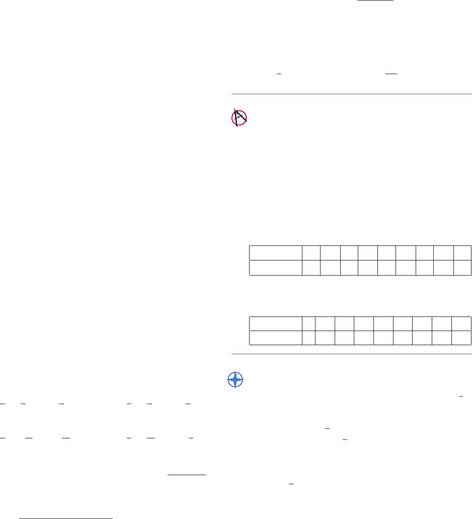
See Figure 4.6 for an illustration of a regular partition for the case where n = 6. On each
subinterval [x
i−1
, x
i
] (for i = 1, 2,...,n), construct a rectangle of height f (x
i
) (the value
x x x x x x
a x
0
x
1
x
2
x
3
x
4
x
5
b x
6
FIGURE 4.6
Regular partition of [a, b]
2.0
y
1.5
1.0
0.5
x
x
4
x
3
x
2
x
1
x
0
FIGURE 4.7
A ≈ A
4
of the function at the right endpoint of the subinterval), as illustrated in Figure 4.7 for the
case where n = 4. It should be clear from Figure 4.7 that the area under the curve A is
roughly the same as the sum of the areas of the four rectangles,
A ≈ f (x
1
)x + f (x
2
)x + f (x
3
)x + f (x
4
)x = A
4
.
In particular, notice that although two of these rectangles enclose more area than that under
the curve and two enclose less area, on the whole, the sum of the areas of the four rectangles
provides an approximation to the total area underthe curve. More generally, if we construct
n rectangles of equal width on the interval [a, b], we have
A ≈ f (x
1
)x + f (x
2
)x +···+ f (x
n
)x
=
n
i=1
f (x
i
)x = A
n
. (3.1)
P1: OSO/OVY P2: OSO/OVY QC: OSO/OVY T1: OSO
MHDQ256-Ch04 MHDQ256-Smith-v1.cls December 13, 2010 21:23
LT (Late Transcendental)
CONFIRMING PAGES
4-17 SECTION 4.3
..
Area 267
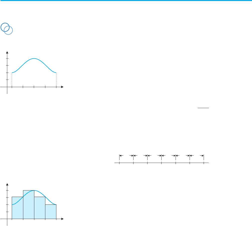
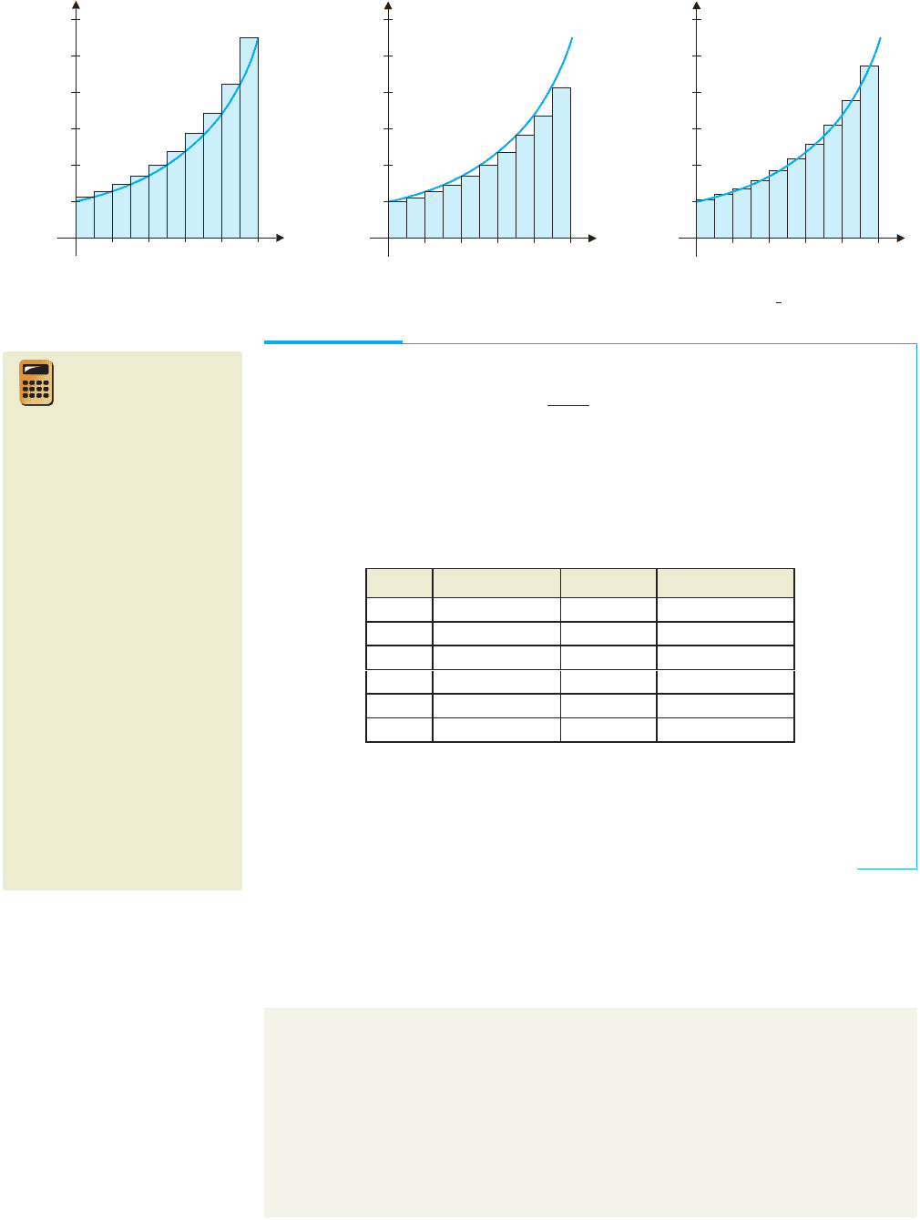
EXAMPLE 3.1 Approximating an Area Using Rectangles
Approximate the area under the curve y = f (x) = 2x −2x
2
on the interval [0, 1],
using (a) 10 rectangles and (b) using 20 rectangles.
y
x
0.5
0.4
0.3
0.2
0.1
0.2
0.4 0.6 0.8 1.0
FIGURE 4.8
A ≈ A
10
Solution (a) The partition divides the interval into 10 subintervals, each of length
x = 0.1, namely [0, 0.1], [0.1, 0.2],...,[0.9, 1.0]. In Figure 4.8, we have drawn in
rectangles of height f (x
i
) on each subinterval [x
i−1
, x
i
] for i = 1, 2,...,10. Notice
that the sum of the areas of the 10 rectangles indicated provides an approximation to the
area under the curve. That is,
A ≈ A
10
=
10
i=1
f (x
i
)x
= [ f (0.1) + f (0.2) +···+ f (1.0)](0.1)
= (0.18 +0.32 +0.42 +0.48 +0.5 +0.48 +0.42 + 0.32 + 0.18 + 0)(0.1)
= 0.33.
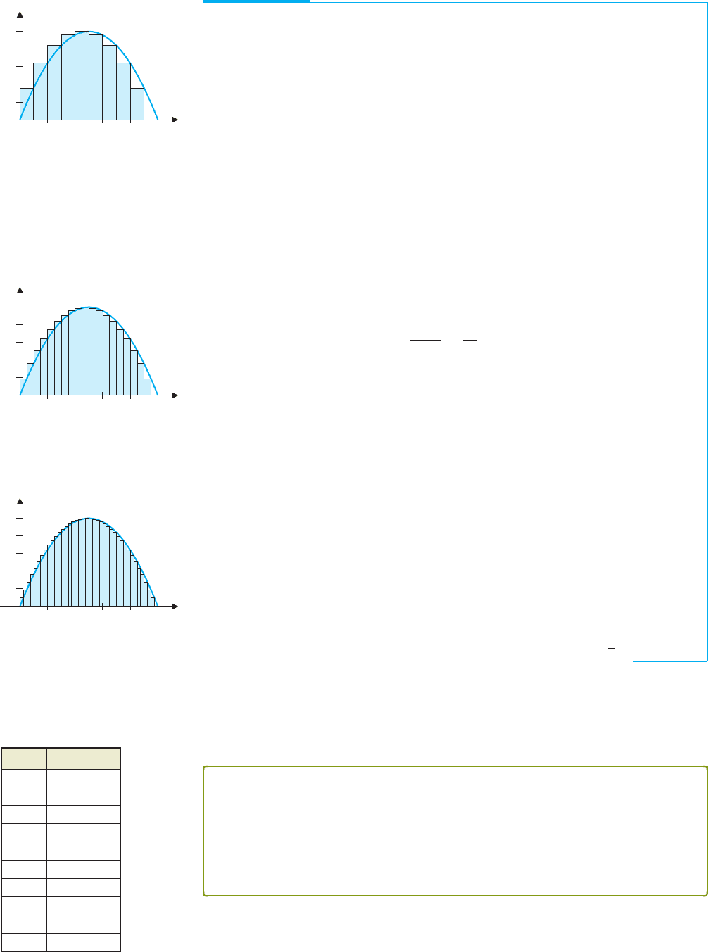
(b) Here, we partition the interval [0, 1] into 20 subintervals, each of width
x =
1 − 0
20
=
1
20
= 0.05.
We then have x
0
= 0, x
1
= 0 + x = 0.05, x
2
= x
1
+ x = 2(0.05) and so on, so that
x
i
= (0.05)i, for i = 0, 1, 2,...,20. From (3.1), the area is then approximately
A ≈ A
20
=
20
i=1
f (x
i
)x =
20
i=1
2x
i
− 2x
2
i
x
=
20
i=1
2[0.05i −(0.05i)
2
](0.05) = 0.3325,
where the details of the calculation are left for the reader. Figure 4.9 shows an
approximation using 20 rectangles and in Figure 4.10, we see 40 rectangles.
y
x
0.5
0.4
0.3
0.2
0.1
0.2
0.4 0.6 0.8 1.0
FIGURE 4.9
A ≈ A
20
y
0.5
0.4
0.3
0.2
0.1
x
0.2
0.4 0.6 0.8 1.0
FIGURE 4.10
A ≈ A
40
n A
n
10 0.33
20 0.3325
30 0.332963
40 0.333125
50 0.3332
60 0.333241
70 0.333265
80 0.333281
90 0.333292
100 0.3333
Based on Figures 4.8–4.10, you should expect that the larger we make n, the better
A
n
will approximate the actual area, A. The obvious drawback to this idea is the length
of time it would take to compute A
n
, for n large. However, your CAS or programmable
calculator can compute these sums for you, with ease. The table shown in the margin
indicates approximate values of A
n
for various values of n.
Notice that as n gets larger and larger, A
n
seems to be approaching
1
3
.
Example 3.1 gives strong evidence that the larger the number of rectangles we use,
the better our approximation of the area becomes. Thinking this through, we arrive at the
following definition of the area under a curve.
DEFINITION 3.1
For a function f defined on the interval [a, b], if f is continuous on [a, b] and
f (x) ≥ 0on[a, b], the area A under the curve y = f (x)on[a, b]isgivenby
A = lim
n→∞
A
n
= lim
n→∞
n
i=1
f (x
i
)x. (3.2)
In example 3.2, we use the limit defined in (3.2) to find the exact area under the curve
from example 3.1.

P1: OSO/OVY P2: OSO/OVY QC: OSO/OVY T1: OSO
MHDQ256-Ch04 MHDQ256-Smith-v1.cls December 13, 2010 21:23
LT (Late Transcendental)
CONFIRMING PAGES
268 CHAPTER 4
..
Integration 4-18
EXAMPLE 3.2 Computing the Area Exactly
Find the area under the curve y = f (x) = 2x −2x
2
on the interval [0, 1].
Solution Here, using n subintervals, we have
x =
1 − 0
n
=
1
n
and so, x
0
= 0, x
1
=
1
n
, x
2
= x
1
+ x =
2
n
and so on. Then, x
i
=
i
n
, for i = 0,
1, 2,...,n. From (3.1), the area is approximately
A ≈ A
n
=
n
i=1
f
i
n
1
n
=
n
i=1
2
i
n
− 2
i
n
2
1
n
=
n
i=1
2
i
n
1
n
−
n
i=1
2
i
2
n
2
1
n
=
2
n
2
n
i=1
i −
2
n
3
n
i=1
i
2
=
2
n
2
n(n +1)
2
−
2
n
3
n(n +1)(2n + 1)
6
From Theorem 2.1 (ii) and (iii).
=
n + 1
n
−
(n + 1)(2n + 1)
3n
2
=
(n + 1)(n − 1)
3n
2
.
Since we have a formula for A
n
, for any n, we can compute various values with ease.
We have
A
200
=
(201)(199)
3(40,000)
= 0.333325,
A
500
=
(501)(499)
3(250,000)
= 0.333332
and so on. Finally, we can compute the limiting value of A
n
explicitly. We have
lim
n→∞
A
n
= lim
n→∞
n
2
− 1
3n
2
= lim
n→∞
1 − 1/n
2
3
=
1
3
.
Therefore, the exact area in Figure 4.8 is 1/3, as we had suspected.
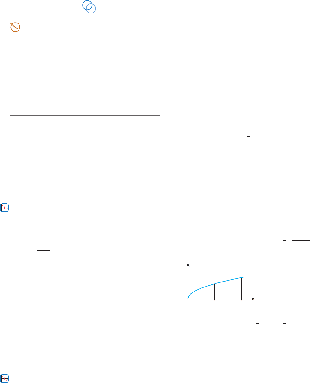
EXAMPLE 3.3 Estimating the Area Under a Curve
Estimate the area under the curve y = f (x) =
√
x +1 on the interval [1, 3].
Solution Here, we have
x =
3 − 1
n
=
2
n
and x
0
= 1, so that
x
1
= x
0
+ x = 1 +
2
n
,
x
2
= 1 +2
2
n
and so on, so that
x
i
= 1 +
2i
n
, for i = 0, 1, 2,...,n.
P1: OSO/OVY P2: OSO/OVY QC: OSO/OVY T1: OSO
MHDQ256-Ch04 MHDQ256-Smith-v1.cls December 13, 2010 21:23
LT (Late Transcendental)
CONFIRMING PAGES
4-19 SECTION 4.3
..
Area 269
Thus, we have from (3.1) that
A ≈ A
n
=
n
i=1
f (x
i
)x =
n
i=1
x
i
+ 1 x
=
n
i=1
1 +
2i
n
+ 1
2
n
=
2
n
n
i=1
2 +
2i
n
.
n A
n
10 3.50595
50 3.45942
100 3.45357
500 3.44889
1000 3.44830
5000 3.44783
We have no formulas like those in Theorem 2.1 for simplifying this last sum (unlike the
sum in example 3.2). Our only choice, then, is to compute A
n
for a number of values of
n using a CAS or programmable calculator. The table shown in the margin lists
approximate values of A
n
. Although we can’t compute the area exactly (as yet), you
should get the sense that the area is approximately 3.4478.
We pause now to define some of the mathematical objects we have been examining.
HISTORICAL
NOTES
Bernhard Riemann
(1826–1866)
A German mathematician who
made important generalizations
to the definition of the integral.
Riemann died at a young age
without publishing many papers,
but each of his papers was highly
influential. His work on
integration was a small portion
of a paper on Fourier series.
Pressured by Gauss to deliver a
talk on geometry, Riemann
developed his own geometry,
which provided a generalization of
both Euclidean and non-Euclidean
geometry. Riemann’s work often
formed unexpected and insightful
connections between analysis and
geometry.
DEFINITION 3.2
Let {x
0
, x
1
,...,x
n
} be a regular partition of the interval [a, b], with
x
i
− x
i−1
= x =
b −a
n
, for all i. Pick points c
1
, c
2
,...,c
n
, where c
i
is any point in
the subinterval [x
i−1
, x
i
], for i = 1, 2,...,n. (These are called evaluation points.)
The Riemann sum for this partition and set of evaluation points is
n
i=1
f (c
i
)x.
So far, we have seen that for a continuous, nonnegative function f, the area under the curve
y = f (x) is the limit of the Riemann sums:
A = lim
n→∞
n
i=1
f (c
i
)x, (3.3)
where c
i
= x
i
, for i = 1, 2,...,n. Surprisingly, for any continuous function f, the limit
in (3.3) is the same for any choice of the evaluation points c
i
∈ [x
i−1
, x
i
] (although the
proof is beyond the level of this course). In examples 3.2 and 3.3, we used the evaluation
points c
i
= x
i
, for each i (the right endpoint of each subinterval). This is usually the most
convenientchoice when working by hand, butdoes not generally produce the most accurate
approximation for a given value of n.
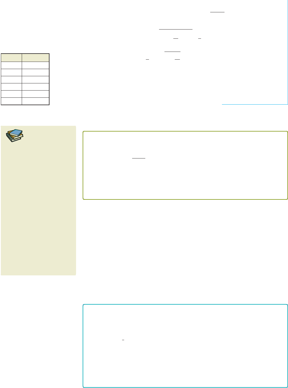
REMARK 3.1
Most often, we cannot compute the limit of Riemann sums indicated in (3.3) exactly
(at least not directly). However, we can always obtain an approximation to the area by
calculating Riemann sums for some large values of n. The most common (and
obvious) choices for the evaluation points c
i
are x
i
(the right endpoint), x
i−1
(the left
endpoint) and
1
2
(x
i−1
+ x
i
) (the midpoint). See Figures 4.11a, 4.11b and 4.11c (on the
following page) for the right endpoint, left endpoint and midpoint approximations,
respectively, for f (x) = 9x
2
+ 2, on the interval [0, 1], using n = 10. You should note
that in this case (as with any increasing function), the rectangles corresponding to the
right endpoint evaluation (Figure 4.11a) give too much area on each subinterval, while
the rectangles corresponding to left endpoint evaluation (Figure 4.11b) give too little
area. We leave it to you to observe that the reverse is true for a decreasing function.
P1: OSO/OVY P2: OSO/OVY QC: OSO/OVY T1: OSO
MHDQ256-Ch04 MHDQ256-Smith-v1.cls December 13, 2010 21:23
LT (Late Transcendental)
CONFIRMING PAGES
270 CHAPTER 4
..
Integration 4-20
y
x
8
0.2
0.4 0.6 0.8 1.0
10
12
6
4
2
x
8
0.2
0.4 0.6 0.8 1.0
10
12
6
4
2
y
x
8
0.2
0.4 0.6 0.8 1.0
10
6
4
2
12
y
FIGURE 4.11a
c
i
= x
i
FIGURE 4.11b
c
i
= x
i−1
FIGURE 4.11c
c
i
=
1
2
(x
i−1
+ x
i
)
EXAMPLE 3.4 Computing Riemann Sums with Different
Evaluation Points
Compute Riemann sums for f (x) =
√
x +1 on the interval [1, 3], for n = 10, 50,
100, 500, 1000 and 5000, using the left endpoint, right endpoint and midpoint of each
subinterval as the evaluation points.
Solution The numbers given in the following table are from a program written for a
programmable calculator. We suggest that you test your own program or one built into
your CAS against these values (rounded off to six digits).
n Left Endpoint Midpoint Right Endpoint
10 3.38879 3.44789 3.50595
50 3.43599 3.44772 3.45942
100 3.44185 3.44772 3.45357
500 3.44654 3.44772 3.44889
1000 3.44713 3.44772 3.44830
5000 3.44760 3.44772 3.44783
TODAY IN
MATHEMATICS
Louis de Branges (1932– )
A French mathematician who
proved the Bieberbach conjecture
in 1985. To solve this famous
70-year-old problem, de Branges
actually proved a related but
much stronger result. In 2004,
de Branges posted on the Internet
what he believes is a proof of
another famous problem, the
Riemann hypothesis. To qualify
for the $1 million prize offered for
the first proof of the Riemann
hypothesis, the result will have
to be verified by expert
mathematicians. However,
de Branges has said, “I am
enjoying the happiness of having a
theory which is in my own hands
and not in that of eventual
readers. I would not want to end
that situation for a million
dollars.”
There are several conclusions to be drawn from these numbers. First, there is good
evidence that all three sets of numbers are converging to a common limit of
approximately 3.4477. Second, even though the limits are the same, the different rules
approach the limit at different rates. You should try computing left and right endpoint
sums for larger values of n, to see that these eventually approach 3.44772, also.
Riemann sums using midpoint evaluation are usually more accurate than left or right
endpoint rules for a given value of n. If you think about the corresponding rectangles, you
may be able to explain why. Finally, notice that the left and right endpoint sums in example
3.4 approach the limit from opposite directions and at about the same rate.
BEYOND FORMULAS
We have now developed a technique for using limits to compute certain areas exactly.
This parallels the derivation of the slope of the tangent line as the limit of the slopes
of secant lines. Recall that this limit became known as the derivative and turned out to
have applications far beyond the slope of a tangent line. Similarly, Riemann sums lead
us to a second major area of calculus, called integration. Based on your experience
with the derivative, do you expect this new limit to solve problems beyond the area of a
region? Do you expect that there will be rules developed to simplify the calculations?
P1: OSO/OVY P2: OSO/OVY QC: OSO/OVY T1: OSO
MHDQ256-Ch04 MHDQ256-Smith-v1.cls December 13, 2010 21:23
LT (Late Transcendental)
CONFIRMING PAGES
4-21 SECTION 4.3
..
Area 271
EXERCISES 4.3
WRITING EXERCISES
1. For many functions, the limit of the Riemann sums is inde-
pendent of the choice of evaluation points. As the number of
partition points gets larger, the distance between the endpoints
gets smaller. For a continuous function f (x), explain why the
difference between the function values at any two points in a
given subinterval will have to get smaller.
2. Rectangles are not the only basic geometric shapes for which
we have an area formula. Discuss how you might approximate
the area under a parabola using circles or triangles. Which
geometric shape do you think is the easiest to use?
In exercises 1–4, list the evaluation points corresponding to the
midpoint of each subinterval, sketch the function and approxi-
mating rectangles and evaluate the Riemann sum.
1. f (x) = x
2
+ 1, (a) [0, 1], n = 4; (b) [0, 2], n = 4
2. f (x) = x
3
− 1, (a) [1, 2], n = 4; (b) [1, 3], n = 4
3. f (x) = sin x, (a) [0,π], n = 4; (b) [0,π], n = 8
4. f (x) = 4 − x
2
, (a) [−1, 1], n = 4; (b) [−3, −1], n = 4
............................................................
In exercises 5–10, approximate the area under the curve on the
given interval using n rectangles and the evaluation rules (a) left
endpoint, (b) midpoint and (c) right endpoint.
5. y = x
2
+ 1on[0, 1], n = 16
6. y = x
2
+ 1on[0, 2], n = 16
7. y =
√
x + 2on[1, 4], n = 16
8. y =
1
x + 2
on [−1, 1], n = 16
9. y = cos x on [0,π/2], n = 50
10. y = x
3
− 1on[−1, 1], n = 100
............................................................
In exercises 11–14, use Riemann sums and a limit to compute
the exact area under the curve.
11. y = x
2
+ 1 on (a) [0, 1], (b) [0, 2], (c) [1, 3]
12. y = x
2
+ 3x on (a) [0, 1], (b) [0, 2], (c) [1, 3]
13. y = 2x
2
+ 1 on (a) [0, 1], (b) [−1, 1], (c) [0, 4]
14. y = 4x
2
− x on (a) [0, 1], (b) [−1, 1], (c) [0, 4]
............................................................
In exercises 15–18, construct a table of Riemann sums as in
example 3.5, to show that sums with right-endpoint, midpoint
and left-endpoint evaluation all converge to the same value as
n → ∞.
15. f (x) = 4 − x
2
, [−2, 2] 16. f (x) = sin x, [0,π/2]
17. f (x) = x
3
− 1, [1, 3] 18. f (x) = x
3
− 1, [−1, 1]
............................................................
In exercises 19–22, graphically determine whether a Riemann
sum with (a) left-endpoint, (b) midpoint and (c) right-endpoint
evaluationpoints will be greater than or less than the area under
the curve y f (x)on[a, b].
19. f (x) is increasing and concave up on [a, b].
20. f (x) is increasing and concave down on [a, b].
21. f (x) is decreasing and concave up on [a, b].
22. f (x) is decreasing and concave down on [a, b].
............................................................
23. For the function f (x) = x
2
on the interval [0, 1], by trial and
error find evaluation points for n = 2 such that the Riemann
sum equals the exact area of 1/3.
24. For the function f (x) =
√
x on the interval [0, 1], by trial and
error find evaluation points for n = 2 such that the Riemann
sum equals the exact area of 2/3.
25. (a) Show that for right-endpoint evaluation on the inter-
val [a, b] with each subinterval of length x = (b − a)/n,
the evaluation points are c
i
= a + ix, for i = 1, 2,...,n.
(b) Find a formula for the evaluation points for midpoint
evaluation.
26. (a) Show that for left-endpoint evaluation on the interval
[a, b] with each subinterval of length x = (b −a)/n, the
evaluation points are c
i
= a + (i − 1)x, for i = 1, 2,...,n.
(b) Find a formula for evaluation points that are one-third of
the way from the left endpoint to the right endpoint.
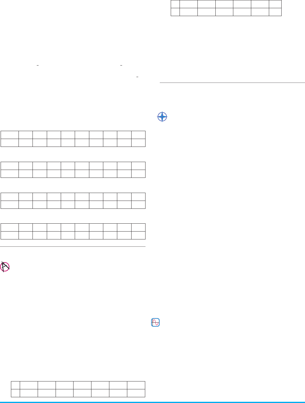
27. In the figure, which area equals lim
n→∞
n
i=1
√
2
1 +i/n
2
n
?
y
x
y 兹x
A
1
A
2
1 2 3 4
28. Which area equals lim
n→∞
n
i=1
1
n
√
1 + 2i
2
n
?
............................................................
In exercises 29–32, use the following definitions. The upper sum
of f on P is given by U(P, f )
n
i1
f (c
i
) x, where f (c
i
) is the
maximum of f on the subinterval [x
i−1
, x
i
]. Similarly, the lower
sum of f on P is given by L(P, f )
n
i1
f (d
i
) x, where f (d
i
)
is the minimum of f on the subinterval [x
i−1
, x
i
].
29. Compute the upper sum and lower sum of f (x) = x
2
on [0, 2]
for the regular partition with n = 4.
30. Computetheuppersumandlowersumof f (x) = x
2
on[−2,2]
for the regular partition with n = 8.
P1: OSO/OVY P2: OSO/OVY QC: OSO/OVY T1: OSO
MHDQ256-Ch04 MHDQ256-Smith-v1.cls December 13, 2010 21:23
LT (Late Transcendental)
CONFIRMING PAGES
272 CHAPTER 4
..
Integration 4-22
31. Find (a) the general upper sum and (b) the general lower sum
for f (x) = x
2
on [0, 2] and show that both sums approach the
same number as n →∞.
32. Repeat exercise 31 for f (x) = x
3
+ 1 on the interval [0, 2].
............................................................
33. The following result has been credited to Archimedes. (See
the historical note on page 325). For the general parabola
y = a
2
− x
2
with −a ≤ x ≤ a, show that the area under the
parabola is
2
3
of the base times the height [that is,
2
3
(2a)(a
2
)].
34. Show that the area under y = ax
2
for 0 ≤ x ≤ b equals
1
3
of
the base times the height.
............................................................
In exercises 35–38, use the given function values to estimate
the area under the curve using left-endpoint and right-endpoint
evaluation.
35.
x 0.0 0.1 0.2 0.3 0.4 0.5 0.6 0.7 0.8
f (x) 2.0 2.4 2.6 2.7 2.6 2.4 2.0 1.4 0.6
36.
x 0.0 0.2 0.4 0.6 0.8 1.0 1.2 1.4 1.6
f (x) 2.0 2.2 1.6 1.4 1.6 2.0 2.2 2.4 2.0
37.
x 1.0 1.1 1.2 1.3 1.4 1.5 1.6 1.7 1.8
f (x) 1.8 1.4 1.1 0.7 1.2 1.4 1.8 2.4 2.6
38.
x 1.0 1.2 1.4 1.6 1.8 2.0 2.2 2.4 2.6
f (x) 0.0 0.4 0.6 0.8 1.2 1.4 1.2 1.4 1.0
APPLICATIONS
39. Economists use a graph called the Lorentz curve to describe
how equally a given quantity is distributed in a given popula-
tion. For example, the gross domestic product (GDP) varies
considerably from country to country. The accompanying data
fromtheEnergyInformationAdministrationshowpercentages
for the 100 top-GDP countries in the world in 2001, arranged
in order of increasing GDP. The data indicate that the first 10
(lowest 10%) countries account for only 0.2% of the world’s
total GDP; the first 20 countries account for 0.4% and so on.
Thefirst99countries account for 73.6%ofthe total GDP.What
percentagedoescountry#100(theUnitedStates)produce?The
Lorentz curve is a plot of y versus x. Graph the Lorentz curve
for these data. Estimate the area between the curve and the
x-axis. (Hint: Notice that the x-values are not equally spaced.
You will need to decide how to handle this.
x 0.1 0.2 0.3 0.4 0.5 0.6 0.7
y 0.002 0.004 0.008 0.014 0.026 0.048 0.085
x 0.8 0.9 0.95 0.98 0.99 1.0
y 0.144 0.265 0.398 0.568 0.736 1.0
40. TheLorentz curve(seeexercise39)can beused to compute the
Gini index, a numerical measure of how inequitable a given
distributionis. Let A
1
equalthe area between the Lorentzcurve
and the x-axis. Construct the Lorentz curve for the situation of
all countries being exactly equal in GDP and let A
2
be the area
between this new Lorentz curve and the x-axis. The Gini index
G equals A
1
divided by A
2
. Explain why 0 ≤ G ≤ 1 and show
that G = 2A
1
. Estimate G for the data in exercise 39.
EXPLORATORY EXERCISES
1. Riemann sums can also be defined on irregular partitions,
for which subintervals are not of equal size. An example
of an irregular partition of the interval [0, 1] is x
0
= 0,
x
1
= 0.2, x
2
= 0.6, x
3
= 0.9, x
4
= 1. Explain why the corre-
sponding Riemann sum would be
f (c
1
)(0.2) + f (c
2
)(0.4) + f (c
3
)(0.3) + f (c
4
)(0.1),
forevaluationpointsc
1
, c
2
, c
3
andc
4
.Identifytheintervalfrom
which each c
i
must be chosen and give examples of evaluation
points. To see why irregular partitions might be useful, con-
sider the function f (x) =
2x if x < 1
x
2
+ 1ifx ≥ 1
on the interval
[0, 2]. One way to approximate the area under the graph of this
function is to compute Riemann sums using midpoint evalua-
tion for n = 10, n = 50, n = 100 and so on. Show graphically
and numerically that with midpoint evaluation, the Riemann
sum with n = 2 gives the correct area on the subinterval [0, 1].
Then explain why it would be wasteful to compute Riemann
sums on this subinterval for larger and larger values of n.A
more efficient strategy would be to compute the areas on [0, 1]
and [1, 2] separately and add them together. The area on [0, 1]
can be computed exactly using a small value of n, while the
area on [1, 2] must be approximated using larger and larger
values of n. Use this technique to estimate the area for f (x)
on the interval [0, 2]. Try to determine the area to within an
error of 0.01 and discuss why you believe your answer is this
accurate.
2. Graph the function f (x) = 1/x for x > 0. We define the area
function g(t) to be the area between this graph and the x-
axis between x = 1 and x = t (for now, assume that t > 1).
Sketch the area that defines g(2) and g(3) and argue that
g(3) > g(2). Explain why the function g(x) is increasing and
hence g
(x) > 0 for x > 1. Further, argue that g
(3) < g
(2).
Explain why g
(x) is a decreasing function. Thus, g
(x) has
the same general properties (positive, decreasing) that f (x)
does. In fact, we will discover in section4.5 that g
(x) = f (x).
To collect some evidence for this result, use Riemann sums
to estimate g(3), g(2.1), g(2.01) and g(2). Use these values to
estimate g
(2) and compare to f (2).