Smith R., Minton R. Calculus
Подождите немного. Документ загружается.


P1: OSO/OVY P2: OSO/OVY QC: OSO/OVY T1: OSO
MHDQ256-Ch04 MHDQ256-Smith-v1.cls December 13, 2010 21:23
LT (Late Transcendental)
CONFIRMING PAGES
4-43 SECTION 4.6
..
Integration by Substitution 293
since F is an antiderivative of f. If you read the expressions on the far left and the far right
sides of (6.1), this suggests that
du =
du
dx
dx.
So, if we cannot compute the integral
h(x) dx directly, we often look for a new variable
u and function f (u) for which
h(x)dx =
f (u(x))
du
dx
dx =
f (u)du,
where the second integral is easier to evaluate than the first.
NOTES
In deciding how to choose a new
variable, there are several things
to look for:
r
terms that are derivatives of
other terms (or pieces thereof)
and
r
terms that are particularly
troublesome. (You can often
substitute your troubles away.)
EXAMPLE 6.2 Using Substitution to Evaluate an Integral
Evaluate
(x
3
+ 5)
100
(3x
2
) dx.
Solution You probably cannot evaluate this as it stands. However, observe that
d
dx
(x
3
+ 5) = 3x
2
,
which is a factor in the integrand. This leads us to make the substitution u = x
3
+ 5, so
that du =
d
dx
(x
3
+ 5) dx = 3x
2
dx. This gives us
(x
3
+ 5)
100
u
100
(3x
2
) dx
du
=
u
100
du =
u
101
101
+ c.
We are not done quite yet. Since we invented the new variable u, we need to convert back
to the original variable x, to obtain
(x
3
+ 5)
100
(3x
2
) dx =
u
101
101
+ c =
(x
3
+ 5)
101
101
+ c.
It’s always a good idea to perform a quick check on the antiderivative. (Remember that
integration and differentiation are inverse processes!) Here, we compute
d
dx
(x
3
+ 5)
101
101
=
101(x
3
+ 5)
100
(3x
2
)
101
= (x
3
+ 5)
100
(3x
2
),
which is the original integrand. This confirms that we have indeed found an
antiderivative.
INTEGRATION BY SUBSTITUTION
Integration by substitution consists of the following general steps, as illustrated in
example 6.2.
r
Choose a new variable u: a common choice is the innermost expression or
“inside” term of a composition of functions. (In example 6.2, note that x
3
+ 5is
the inside term of (x
3
+ 5)
100
.)
r
Compute du =
du
dx
dx.
r
Replace all terms in the original integrand with expressions involving u and du.
r
Evaluate the resulting (u) integral. If you still can’t evaluate the integral, you
may need to try a different choice of u.
r
Replace each occurrence of u in the antiderivative with the corresponding
expression in x.

P1: OSO/OVY P2: OSO/OVY QC: OSO/OVY T1: OSO
MHDQ256-Ch04 MHDQ256-Smith-v1.cls December 13, 2010 21:23
LT (Late Transcendental)
CONFIRMING PAGES
294 CHAPTER 4
..
Integration 4-44
Always keep in mind that finding antiderivatives is the reverse process of finding
derivatives. In example 6.3, we are not so fortunate as to have the exact derivative we want
in the integrand.
EXAMPLE 6.3 Using Substitution: A Power Function Inside a Cosine
Evaluate
x cos x
2
dx.
Solution Notice that
d
dx
x
2
= 2x.
While we don’t quite have a factor of 2x in the integrand, we can always push constants
back and forth past an integral sign and rewrite the integral as
x cos x
2
dx =
1
2
2x cos x
2
dx.
We now substitute u = x
2
, so that du = 2xdxand we have
x cos x
2
dx =
1
2
cos x
2
cos u
(2x)dx
du
=
1
2
cosudu=
1
2
sinu + c =
1
2
sin x
2
+ c.
Again, as a check, observe that
d
dx
1
2
sin x
2
=
1
2
cos x
2
(2x) = x cosx
2
,
which is the original integrand.
EXAMPLE 6.4 Using Substitution: A Trigonometric Function
Inside a Power
Evaluate
(3tan x + 4)
5
sec
2
xdx.
Solution As with most integrals, you probably can’t evaluate this one as it stands.
However, observe that there’s a tan x term and a factor of sec
2
x in the integrand and that
d
dx
tan x = sec
2
x. Thus, we let u = 3tan x + 4, so that du = 3sec
2
xdx. We then have
(3tan x + 4)
5
sec
2
xdx=
1
3
(3tan x + 4)
5
u
5
(3sec
2
x) dx
du
=
1
3
u
5
du =
1
3
u
6
6
+ c
=
1
18
(3tan x + 4)
6
+ c.
Sometimes you will need to look a bit deeper into an integral to see terms that are
derivatives of other terms, as in example 6.5.
EXAMPLE 6.5 Using Substitution: A Root Function Inside a Sine
Evaluate
sin
√
x
√
x
dx.
Solution This integral is not especially obvious. It never hurts to try something,
though. If you had to substitute for something, what would you choose? You might

P1: OSO/OVY P2: OSO/OVY QC: OSO/OVY T1: OSO
MHDQ256-Ch04 MHDQ256-Smith-v1.cls December 13, 2010 21:23
LT (Late Transcendental)
CONFIRMING PAGES
4-45 SECTION 4.6
..
Integration by Substitution 295
notice that sin
√
x = sin x
1/2
and letting u =
√
x = x
1/2
(the “inside”), we get
du =
1
2
x
−1/2
dx =
1
2
√
x
dx. Since there is a factor of
1
√
x
in the integrand, we can
proceed. We have
sin
√
x
√
x
dx = 2
sin
√
x
sin u
1
2
√
x
dx
du
= 2
sinudu=−2 cosu + c =−2cos
√
x +c.
So far, every one of our examples has been solved by spotting a term in the integrand
that was the derivative of another term. We present an integral now where this is not the
case, but where a substitution is made to deal with a particularly troublesome term in the
integrand.
EXAMPLE 6.6 A Substitution That Lets You Expand the Integrand
Evaluate
x
√
2 − xdx.
Solution You certainly cannot evaluate this as it stands and if you look for terms that
are derivatives of other terms, you will come up empty-handed. The real problem here is
that there is a square root of a sum (or difference) in the integrand. A reasonable step
would be to substitute for the expression under the square root. We let u = 2 − x,so
that du =−dx. That doesn’t seem so bad, but what are we to do with the extra x in the
integrand? Well, since u = 2 − x, it follows that x = 2 − u. Making these substitutions
in the integral, we get
x
√
2 − xdx = (−1)
x
2 −u
√
2 − x
√
u
(−1)dx
du
=−
(2 − u)
√
udu.
While we can’t evaluate this integral directly, if we multiply out the terms, we get
x
√
2 − xdx =−
(2 − u)
√
udu
=−
(2u
1/2
− u
3/2
)du
=−2
u
3/2
3
2
+
u
5/2
5
2
+ c
=−
4
3
u
3/2
+
2
5
u
5/2
+ c
=−
4
3
(2 − x)
3/2
+
2
5
(2 − x)
5/2
+ c.
You should check the validity of this antiderivative via differentiation.
Substitution in Definite Integrals
Thereis only oneslightdifferenceinusing substitution forevaluatinga definiteintegral:you
must also change the limits of integration to correspond to the new variable. The procedure
here is then precisely the same as that used for examples 6.2 through 6.6, except that when
you introduce the new variable u, the limits of integration change from x = a and x = b to
the corresponding limits for u: u = u(a) and u = u(b). We have
b
a
f (u(x))u
(x)dx =
u(b)
u(a)
f (u)du.

P1: OSO/OVY P2: OSO/OVY QC: OSO/OVY T1: OSO
MHDQ256-Ch04 MHDQ256-Smith-v1.cls December 13, 2010 21:23
LT (Late Transcendental)
CONFIRMING PAGES
296 CHAPTER 4
..
Integration 4-46
EXAMPLE 6.7 Using Substitution in a Definite Integral
Evaluate
2
1
x
3
√
x
4
+ 5 dx.
Solution Of course, you probably can’t evaluate this as it stands. However, since
d
dx
(x
4
+ 5) = 4x
3
, we make the substitution u = x
4
+ 5, so that du = 4x
3
dx. For the
limits of integration, note that when x = 1,
u = x
4
+ 5 = 1
4
+ 5 = 6
and when x = 2, u = x
4
+ 5 = 2
4
+ 5 = 21.
We now have
2
1
x
3
x
4
+ 5 dx =
1
4
2
1
x
4
+ 5
√
u
(4x
3
)dx
du
=
1
4
21
6
√
udu
=
1
4
u
3/2
3
2
21
6
=
1
4
2
3
(21
3/2
− 6
3/2
).
Notice that because we changed the limits of integration to match the new variable,
we did not need to convert back to the original variable, as we do when we make a
substitution in an indefinite integral. (Note that, if we had switched the variables back,
we would also have needed to switch the limits of integration back to their original
values before evaluating!)
CAUTION
You must change the limits of
integration as soon as you
change variables!
It may have occurred to you that you could use a substitution in a definite integral only
to find an antiderivative and then switch back to the original variable to do the evaluation.
Although this method will work for many problems, we recommend that you avoid it, for
several reasons. First, changing the limits of integration is not very difficult and results in
a much more readable mathematical expression. Second, in many applications requiring
substitution, you will need to change the limits of integration, so you might as well get used
to doing so now.
EXAMPLE 6.8 Substitution in a Definite Integral
Involving a Trigonometric Function
Compute
15
0
t sin(−t
2
/2)dt.
Solution As always, we look for terms that are derivatives of other terms. Here, you
should notice that
d
dt
(
−t
2
2
) =−t. So, we set u =−
t
2
2
and compute du =−tdt. For the
upper limit of integration, we have that t = 15 corresponds to u =−
(15)
2
2
=−
225
2
.For
the lower limit, we have that t = 0 corresponds to u = 0. This gives us
15
0
t sin(−t
2
/2)dt =−
15
0
[sin(−t
2
/2)]
sinu
(−t) dt
du
=−
−225/2
0
sinudu= cosu
−112.5
0
= cos(−112.5) − 1.
EXERCISES 4.6
WRITING EXERCISES
1. Itisneverwrong tomakeasubstitutioninanintegral,butsome-
times it isnot very helpful. For example, using the substitution
u = x
2
, you can correctly conclude that
x
3
x
2
+ 1 dx =
1
2
u
√
u + 1 du,
but the new integral is no easier than the original integral. Find
a better substitution and evaluate this integral.
2. It is not uncommon for students learning substitution to
use incorrect notation in the intermediate steps. Be aware
of this—it can be harmful to your grade! Carefully exam-
ine the following string of equalities and find each mistake.

P1: OSO/OVY P2: OSO/OVY QC: OSO/OVY T1: OSO
MHDQ256-Ch04 MHDQ256-Smith-v1.cls December 13, 2010 21:23
LT (Late Transcendental)
CONFIRMING PAGES
4-47 SECTION 4.6
..
Integration by Substitution 297
Using u = x
2
,
2
0
x sin x
2
dx =
2
0
(sinu)xdx=
2
0
(sinu)
1
2
du
=−
1
2
cosu
2
0
=−
1
2
cos x
2
2
0
=−
1
2
cos4 +
1
2
.
The final answer is correct, but because of several errors, this
work would not earn full credit. Discuss each error and write
this in a way that would earn full credit.
3. Suppose that an integrandhas a term of the form sin( f (x)). For
example, suppose you are trying to evaluate
x
2
sin(x
3
)dx.
Discuss why you should immediately try the substitution
u = f (x).
4. Suppose that an integrandhas a composite function of the form
f (g(x)). Explain why you should look to see if the integrand
also has the term g
(x). Discuss possible substitutions.
In exercises 1–4, use the given substitution to evaluate the indi-
cated integral.
1.
x
2
x
3
+ 2 dx, u = x
3
+ 2
2.
x
3
(x
4
+ 1)
−2/3
dx, u = x
4
+ 1
3.
(
√
x + 2)
3
√
x
dx, u =
√
x + 2
4.
sin x cos xdx, u = sin x
............................................................
In exercises 5–28, evaluate the indicated integral.
5.
x
3
x
4
+ 3dx 6.
√
1 + 10xdx
7.
sin x
√
cos x
dx 8.
sin
3
x cos xdx
9.
t
2
cost
3
dt 10.
sint (cost + 3)
3/4
dt
11.
sec
2
x cos(tan x) dx 12.
x csc x
2
cot x
2
dx
13.
cos
√
x
√
x
dx 14.
cos(1/x)
x
2
dx
15.
cos3x
(sin3x +1)
3
dx 16.
sec
2
x
√
tan xdx
17.
1
√
u (
√
u + 1)
2
du 18.
v
√
v
2
+ 4
dv
19.
4
x
2
(2/x + 1)
3
dx 20.
2x
(x + 1)
3
dx
21.
9x
2
(3 − x)
4
dx 22.
x
2
sec
2
x
3
dx
23.
√
4x
5
− x
4
x
2
dx 24.
x
3
√
1 − x
4
dx
25.
2t + 3
(t + 7)
3
dt 26.
t
2
3
√
t + 3
dt
27.
1
1 +
√
x
dx 28.
1
(1 +
√
x)
3
dx
............................................................
In exercises 29–36, evaluate the definite integral.
29.
2
0
x
x
2
+ 1 dx 30.
3
1
x sin(π x
2
)dx
31.
1
−1
t
(t
2
+ 1)
2
dt 32.
π
2
0
cos
√
t
√
t
dt
33.
1
0
x
2
cos x
3
dx 34.
π/4
π/8
csc2x cot2xdx
35.
4
1
x − 1
√
x
dx 36.
1
0
x
√
x
2
+ 1
dx
............................................................
In exercises 37–40, name the method by evaluating the integral
exactly, if possible, or estimating it numerically.
37. (a)
π
0
sin x
2
dx (b)
π
0
x sin x
2
dx
38. (a)
1
−1
x
x
2
+ 4dx (b)
1
−1
x
2
+ 4dx
39. (a)
2
0
4x
2
(x
2
+ 1)
2
dx (b)
2
0
4x
(x
2
+ 1)
2
dx
40. (a)
π/4
0
sec xdx (b)
π/4
0
sec
2
xdx
............................................................
In exercises 41–44, make the indicated substitution for an un-
specified function f (x).
41. u = x
2
for
2
0
xf(x
2
)dx
42. u = x
3
for
2
1
x
2
f (x
3
)dx
43. u = sin x for
π/2
0
(cos x) f (sin x)dx
44. u =
√
x for
4
0
f (
√
x)
√
x
dx
............................................................
45. A function f is said to be even if f (−x) = f (x) for all x.
A function f is said to be odd if f (−x) =−f (x). Sup-
pose that f is continuous for all x. Show that if f is even,
then
a
−a
f (x) dx = 2
a
0
f (x) dx. Also, if f is odd, show that
a
−a
f (x) dx = 0.
46. Assume that f is periodic with period T; that is,
f (x +T ) = f (x)forallx.Showthat
T
0
f (x) dx =
a+T
a
f (x) dx
for any real number a. (Hint: First, work with 0 ≤ a ≤ T.)
47. (a) For the integral I =
10
0
√
x
√
x +
√
10 − x
dx, use a substi-
tution to showthat I =
10
0
√
10 − x
√
x +
√
10 − x
dx.Use these
two representations of I to evaluate I.
(b) Generalize to I =
a
0
f (x)
f (x) + f (a − x)
dx for any pos-
itive, continuous function f and then quickly evaluate
π/2
0
sin x
sin x + cos x
dx.

P1: OSO/OVY P2: OSO/OVY QC: OSO/OVY T1: OSO
MHDQ256-Ch04 MHDQ256-Smith-v1.cls December 13, 2010 21:23
LT (Late Transcendental)
CONFIRMING PAGES
298 CHAPTER 4
..
Integration 4-48
48. (a) For I =
4
2
sin
2
(9 − x)
sin
2
(9 − x) + sin
2
(x + 3)
dx, use the
substitution u = 6 − x to show that
I =
4
2
sin
2
(x + 3)
sin
2
(9 − x) + sin
2
(x + 3)
dx and evaluate I.
(b) Generalize to
4
2
f (9 − x)
f (9 − x) + f (x + 3)
dx, for any posi-
tive, continuous function f on [2, 4].
49. Evaluate
2
0
f (x + 4)
f (x + 4) + f (6 − x)
dx for any positive, con-
tinuous function f on [0, 2].
50. (a) Foru = x
1/6
,showthat
1
x
5/6
+ x
2/3
dx = 6
u
u + 1
du.
(b) Foru = x
1/6
,showthat
1
√
x +
3
√
x
dx = 6
u
3
u + 1
du.
(c) Generalize to
1
x
(p+1)/q
+ x
p/q
dx for positive integers p
and q.
51. Find each mistake in the following calculations and then
show how to correctly do the substitution. Start with
1
−2
4x
4
dx =
1
−2
x(4x
3
)dx and then use the substitution
u = x
4
with du = 4x
3
dx. Then
1
−2
x(4x
3
)dx =
1
16
u
1/4
du =
4
5
u
5/4
u=1
u=16
=
4
5
−
32
5
=−
18
5
52. Find each mistake in the following calculations and then
show how to correctly do the substitution. Start with
π
0
cos
2
xdx=
π
0
cos x(cos x)dx and then use the substitu-
tion u = sin x with du = cos xdx. Then
π
0
cos x(cos x)dx =
0
0
1 − u
2
du = 0
APPLICATIONS
53. The voltage in an AC (alternating current) circuit is given by
V (t) = V
p
sin(2π ft), where f is the frequency. A voltmeter
does not indicate the amplitude V
p
. Instead, the voltmeter
reads the root-mean-square (rms), the square root of the aver-
age value of the square of the voltage over one cycle. That
is, rms =
f
1/ f
0
V
2
(t)dt. Use the trigonometric identity
sin
2
x =
1
2
−
1
2
cos2x to show that rms = V
p
/
√
2.
54. Graph y = f (t) and find the root-mean-square of
f (t) =
⎧
⎨
⎩
−1if−2 ≤ t < −1
t if −1 ≤ t ≤ 1
1if1< t ≤ 2
,
where rms =
1
4
2
−2
f
2
(t)dt.
EXPLORATORY EXERCISES
1. A predator-prey system is a set of differentialequations mod-
eling the change in population of interacting species of organ-
isms. A simple model of this type is
x
(t) = x(t)[a − by(t)]
y
(t) = y(t)[dx(t) −c]
for positive constants a, b, c and d. Both equations include a
term of the form x(t)y(t), which is intended to represent the
result of confrontations between the species. Noting that the
contributionofthistermis negativeto x
(t)butpositiveto y
(t),
explainwhy it mustbethat x(t)represents the populationofthe
preyand y(t) the population of the predator. If x(t) = y(t) = 0,
compute x
(t) and y
(t). In this case, will x and y increase,
decrease or stay constant? Explain why thismakes sense phys-
ically. Determine x
(t) and y
(t) and the subsequent change in
x and y at the so-called equilibrium point x = c/d, y = a/b.
If the population is periodic, we can show that the equilibrium
point gives the average population (evenif the populationdoes
not remain constant). To do so, note that
x
(t)
x(t)
= a − by(t).
Integrating both sides of this equation from t = 0
to t = T [the period of x(t) and y(t)], we get
T
0
x
(t)
x(t)
dt =
T
0
adt−
T
0
by(t)dt. Assuming that x(t)
has period T,wehavex(T ) = x(0) and so, the integral on
the left hand side equals 0. Thus, 0 = aT −
T
0
by(t) dt. Fi-
nally, rearrangeterms toshow that 1/T
T
0
y(t) dt = a/b; that
is, the average value of the population y(t) is the equilibrium
value y = a/b. Similarly, show that the average value of the
population x(t) is the equilibrium value x = c/d.
2. Define the Dirac delta δ(x) to have the defining property
b
−a
δ(x)dx = 1 for any a, b > 0. Assuming that δ(x) acts like
acontinuousfunction(thisisasignificantissue!),usethisprop-
erty to evaluate (a)
1
0
δ(x − 2) dx, (b)
1
0
δ(2x − 1) dx and (c)
1
−1
δ(2x)dx. Assuming that it applies, use the Fundamental
Theorem of Calculus to prove that δ(x) = 0 for all x = 0 and
to prove that δ(x) is unbounded in [−1, 1]. What do you find
troublesome about this? Do you think that δ(x) is really a con-
tinuous function, or even a function at all?
3. Suppose that f is a continuous function such that for
all x, f (2x) = 3 f (x) and f (x +
1
2
) =
1
3
+ f (x). Compute
1
0
f (x) dx.
4.7 NUMERICAL INTEGRATION
Thus far, our development of the integral has paralleled our development of the derivative.
In both cases, we began with a limit definition that was difficult to use for calculation and
P1: OSO/OVY P2: OSO/OVY QC: OSO/OVY T1: OSO
MHDQ256-Ch04 MHDQ256-Smith-v1.cls December 13, 2010 21:23
LT (Late Transcendental)
CONFIRMING PAGES
4-49 SECTION 4.7
..
Numerical Integration 299
then proceeded to develop simplified rules for calculation. At this point, you should be able
to find the derivative of nearly any function you can write down. You might expect that with
a few more rules you will be able to do the same for integrals. Unfortunately, this is not
the case. There are many functions for which no elementary antiderivative is available. (By
elementary antiderivative, we mean anantiderivative expressible in terms of the elementary
functions with which you are familiar: the algebraic and trigonometric functions, as well as
the exponential and logarithmic functions that we’ll introduce in Chapter 6.) For instance,
2
0
cos(x
2
) dx
cannot be calculated exactly, since cos(x
2
) does not have an elementary antiderivative. (Try
to find one, but don’t spend much time on it.)
In fact, most definite integrals cannot be calculated exactly. When we can’t compute
the value of an integral exactly, we do the next best thing: we approximate its value numer-
ically. In this section, we develop three methods of approximating definite integrals. None
will replace the built-in integration routine on your calculator or computer. However, by
exploring these methods, you will gain a basic understanding of some of the ideas behind
more sophisticated numerical integration routines.
Since a definite integral is the limit of a sequence of Riemann sums, any Riemann sum
serves as an approximation of the integral,
b
a
f (x) dx ≈
n
i=1
f (c
i
)x,
where c
i
is any point chosen from the subinterval [x
i−1
, x
i
], for i = 1, 2,...,n. Further,
the larger n is, the better the approximation tends to be. The most common choice of the
evaluation points c
1
, c
2
,...,c
n
leads to a method called the Midpoint Rule:
b
a
f (x) dx ≈
n
i=1
f (c
i
)x,
where c
i
is the midpoint of the subinterval [x
i−1
, x
i
],
c
i
=
1
2
(x
i−1
+ x
i
), for i = 1, 2,...,n.
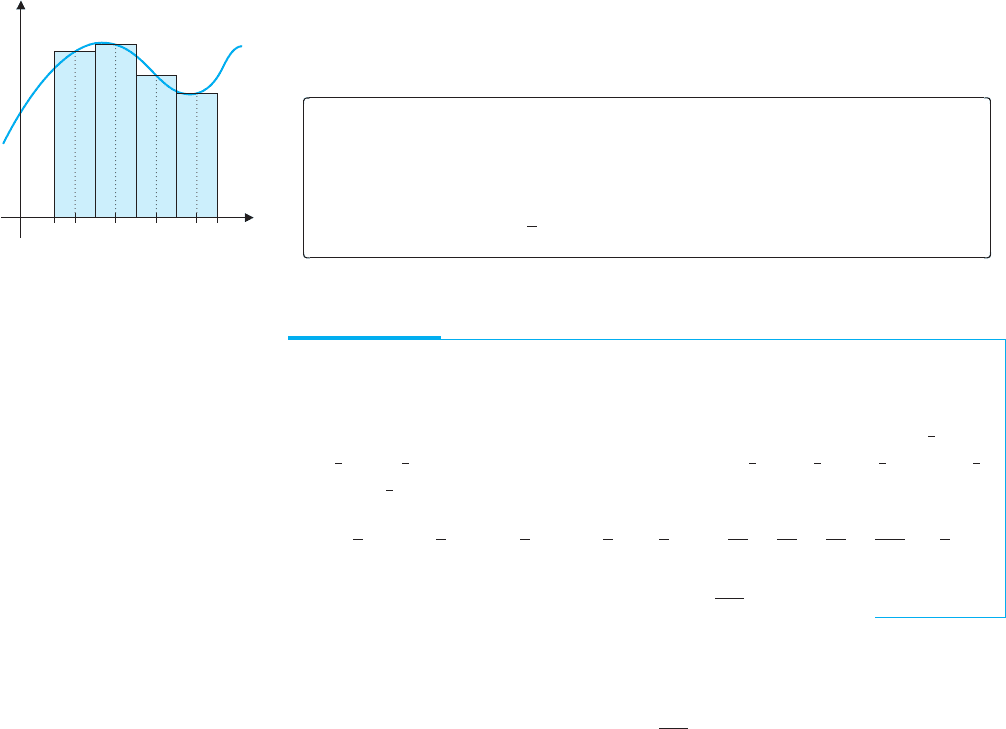
We illustrate this approximation for the case where f (x) ≥ 0on[a, b], in Figure 4.26.
x
y
c
4
c
3
c
2
c
1
a b
FIGURE 4.26
Midpoint Rule
EXAMPLE 7.1 Using the Midpoint Rule
Write out the Midpoint Rule approximation of
1
0
3x
2
dx with n = 4.
Solution For n = 4, the regular partition of the interval [0, 1] is x
0
= 0, x
1
=
1
4
,
x
2
=
1
2
, x
3
=
3
4
and x
4
= 1. The midpoints are then c
1
=
1
8
, c
2
=
3
8
, c
3
=
5
8
and c
4
=
7
8
.
With x =
1
4
, the Riemann sum is then
f
1
8
+ f
3
8
+ f
5
8
+ f
7
8
1
4
=
3
64
+
27
64
+
75
64
+
147
64
1
4
=
252
256
= 0.984375.
Of course, from the Fundamental Theorem, the exact value of the integral in
example 7.1 is
1
0
3x
2
dx =
3x
3
3
1
0
= 1.
So, our approximation in example 7.1 is not especially accurate. To obtain greater accuracy,
notice that you could always compute an approximation using more rectangles. You can

P1: OSO/OVY P2: OSO/OVY QC: OSO/OVY T1: OSO
MHDQ256-Ch04 MHDQ256-Smith-v1.cls December 13, 2010 21:23
LT (Late Transcendental)
CONFIRMING PAGES
300 CHAPTER 4
..
Integration 4-50
simplify this process by writing a simple program for your calculator or computer to im-
plement the Midpoint Rule. A suggested outline for such a program follows.
MIDPOINT RULE
1. Store f (x), a, b and n.
2. Compute x =
b −a
n
.
3. Compute c
1
= a +
x
2
and start the sum with f (c
1
).
4. Compute the next c
i
= c
i−1
+ x and add f (c
i
) to the sum.
5. Repeat step 4 until i = n [i.e., perform step 4 a total of (n − 1) times].
6. Multiply the sum by x.
EXAMPLE 7.2 Using a Program for the Midpoint Rule
Repeat example 7.1 using a program to compute the Midpoint Rule approximations for
n = 8, 16, 32, 64 and 128.
Solution You should confirm the values in the following table. We include a column
displaying the error in the approximation for each n (i.e., the difference between the
exact value of 1 and the approximate values).
n Midpoint Rule Error
4 0.984375 0.015625
8 0.99609375 0.00390625
16 0.99902344 0.00097656
32 0.99975586 0.00024414
64 0.99993896 0.00006104
128 0.99998474 0.00001526
You should note that each time the number of steps is doubled, the error is reduced
approximately by a factor of 4. Although this precise reduction in error will not occur
with all integrals, this rate of improvement in the accuracy of the approximation is
typical of the Midpoint Rule.
Of course, we won’t know the error in a Midpoint Rule approximation, except where
we know the value of the integral exactly. We started with a simple integral, whose value
we knew exactly, so that you could get a sense of how accurate the Midpoint Rule approxi-
mation is.
Note that in example 7.3, we can’t compute an exact value of the integral, since we do
not know an antiderivative for the integrand.
EXAMPLE 7.3 Finding an Approximation with a Given Accuracy
Use the Midpoint Rule to approximate
2
0
√
x
2
+ 1 dx accurate to three decimal places.
Solution To obtain the desired accuracy, we continue increasing n until it appears
unlikely the third decimal will change further. (The size of n will vary substantially from
integral to integral.) You should confirm the numbers in the accompanying table.
From the table, we can make the reasonable approximation
2
0
x
2
+ 1 dx ≈ 2.958.
While this is reasonable, note that there is no guarantee that the digits shown are correct.
To get a guarantee, we will need the error bounds derived later in this section.
n Midpoint Rule
10 2.95639
20 2.95751
30 2.95772
40 2.95779
P1: OSO/OVY P2: OSO/OVY QC: OSO/OVY T1: OSO
MHDQ256-Ch04 MHDQ256-Smith-v1.cls December 13, 2010 21:23
LT (Late Transcendental)
CONFIRMING PAGES
4-51 SECTION 4.7
..
Numerical Integration 301
REMARK 7.1
Computer and calculator programs that estimate the value of an integral face the same
challenge we did in example 7.3—that is, knowing when a given approximation is
good enough. Such software generally includes sophisticated algorithms for
estimating the accuracy of its approximations. You can find an introduction to such
algorithms in most texts on numerical analysis.
Another important reason for pursuing numerical methods is for the case where we
don’tknowthefunction that we’retryingto integrate.That’s right: we oftenknowonlysome
values of a function at a collection of points, while a symbolic representation of a function
is unavailable. This is often the case in the physical and biological sciences and engineering,
where the only information available about a function comes from measurements made at
a finite number of points.
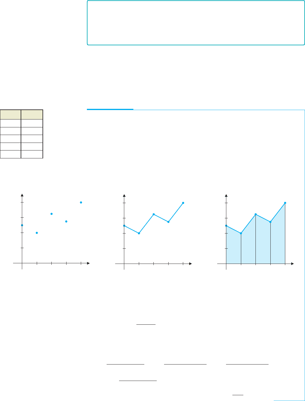
x f (x)
0.0 1.0
0.25 0.8
0.5 1.3
0.75 1.1
1.0 1.6
EXAMPLE 7.4 Estimating an Integral from a Table of Function Values
Estimate
1
0
f (x) dx, where we have values of the unknown function f (x)asgivenin
the table shown in the margin.
Solution Approaching the problem graphically, we have five data points. (See
Figure 4.27a.) How can we estimate the area under the curve from five points?
Conceptually, we have two tasks. First, we need a reasonable way to connect the given
points. Second, we need to compute the area of the resulting region. The most obvious
way to connect the dots is with straight-line segments as in Figure 4.27b.
x
0.4
0.8
1.2
1.6
1.00
0.750.500.25
y
x
0.4
0.8
1.2
1.6
1.00
0.750.500.25
y
x
0.4
0.8
1.2
1.6
1.00
0.750.500.25
y
FIGURE 4.27a FIGURE 4.27b FIGURE 4.27c
Data from an unknown function Connecting the dots Four trapezoids
Notice that the region bounded by the graph and the x-axis on the interval [0, 1]
consists of four trapezoids. (See Figure 4.27c.)
It’s an easy exercise to show that the area of a trapezoid with sides h
1
and h
2
and
base b is given by
h
1
+ h
2
2
b. (Think of this as the average of the areas of the
rectangle whose height is the value of the function at the left endpoint and the rectangle
whose height is the value of the function at the right endpoint.)
The total area of the four trapezoids is then
f (0) + f (0.25)
2
0.25 +
f (0.25) + f (0.5)
2
0.25 +
f (0.5) + f (0.75)
2
0.25
+
f (0.75) + f (1)
2
0.25
= [ f (0) +2 f (0.25) +2 f (0.5) +2 f (0.75) + f (1)]
0.25
2
= 1.125.
P1: OSO/OVY P2: OSO/OVY QC: OSO/OVY T1: OSO
MHDQ256-Ch04 MHDQ256-Smith-v1.cls December 13, 2010 21:23
LT (Late Transcendental)
CONFIRMING PAGES
302 CHAPTER 4
..
Integration 4-52
Moregenerally,foranycontinuousfunction f definedontheinterval[a,b],wepartition
[a, b] as follows:
a = x
0
< x
1
< x
2
< ···< x
n
= b,
where the points in the partition are equally spaced, with spacing x =
b −a
n
. On each
subinterval [x
i−1
, x
i
], approximate the area under the curve by the area of the trapezoid
whose sides have length f (x
i−1
) and f (x
i
), as indicated in Figure 4.28. The area under the
curve on the interval [x
i−1
, x
i
] is then approximately
A
i
≈
1
2
[ f (x
i−1
) + f (x
i
)]x,
for each i = 1, 2,...,n. Adding together the approximations for the area under the curve
on each subinterval, we get that
b
a
f (x) dx ≈
f (x
0
) + f (x
1
)
2
+
f (x
1
) + f (x
2
)
2
+···+
f (x
n−1
) + f (x
n
)
2
x
=
b −a
2n
[ f (x
0
) + 2 f (x
1
) + 2 f (x
2
) +···+2 f (x
n−1
) + f (x
n
)].
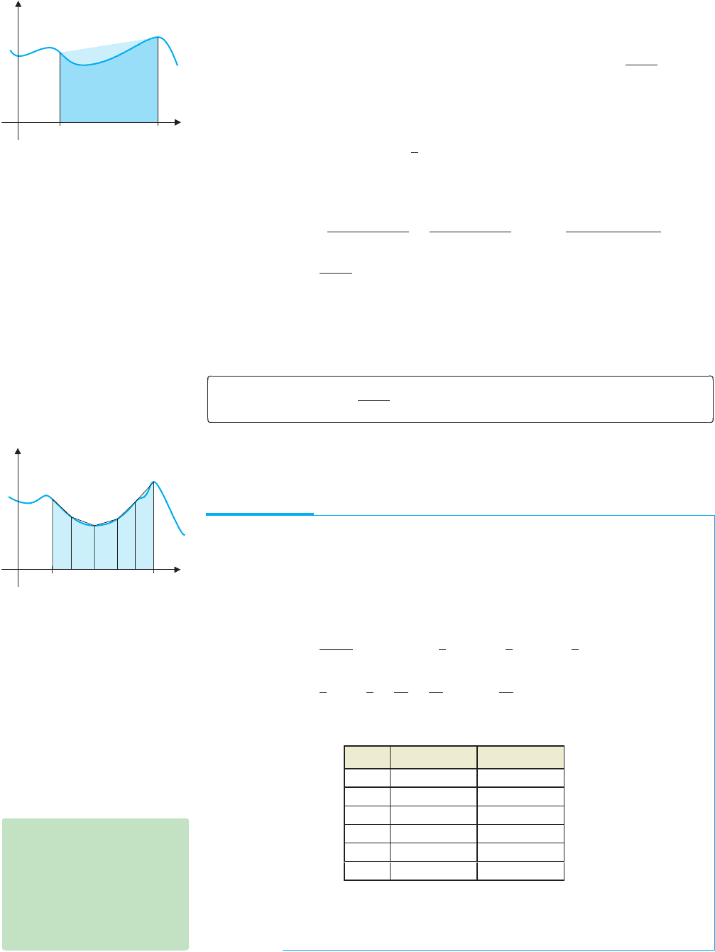
We illustrate this in Figure 4.29. Notice that each of the middle terms is multiplied by 2,
since each one is used in two trapezoids, once as the height of the trapezoid at the right
endpoint and once as the height of the trapezoid at the left endpoint. We refer to this as the
(n + 1)-point Trapezoidal Rule, T
n
( f ),
b
a
f (x) dx ≈ T
n
( f ) =
b −a
2n
[ f (x
0
) + 2 f (x
1
) + 2 f (x
2
) +···+2 f (x
n−1
) + f (x
n
)].
One way to write a program for the Trapezoidal Rule is to add together
Trapezoidal Rule
[ f (x
i−1
) + f (x
i
)] for i = 1, 2,...,n and then multiply by x/2. As discussed in the ex-
ercises, an alternative is to add together the Riemann sums using left- and right-endpoint
evaluations, and then divide by 2.
y
x
x
i
y = f(x)
f(x
i
)
x
i 1
f(x
i 1
)
−
−
FIGURE 4.28
Trapezoidal Rule
y
x
b
y = f(x)
a
FIGURE 4.29
The (n + 1)-point
Trapezoidal Rule
EXAMPLE 7.5 Using the Trapezoidal Rule
Compute the Trapezoidal Rule approximations with n = 4 (by hand) and n = 8, 16,
32, 64 and 128 (using a program) for
1
0
3x
2
dx.
Solution As we saw in examples 7.1 and 7.2, the exact value of this integral is 1. For
the Trapezoidal Rule with n = 4, we have
T
4
( f ) =
1 − 0
(2)(4)
f (0) +2 f
1
4
+ 2 f
1
2
+ 2 f
3
4
+ f (1)
=
1
8
0 +
3
8
+
12
8
+
27
8
+ 3
=
66
64
= 1.03125.
Using a program, you can easily get the values in the accompanying table.
n T
n
( f ) Error
4 1.03125 0.03125
8 1.0078125 0.0078125
16 1.00195313 0.00195313
32 1.00048828 0.00048828
64 1.00012207 0.00012207
128 1.00003052 0.00003052
NOTES
Since the Trapezoidal Rule
formula is an average of two
Riemann sums, we have
b
a
f (x)dx = lim
n→∞
T
n
( f ).
We have included a column showing the error (the absolute value of the difference
between the exact value of 1 and the approximate value). Notice that (as with the
Midpoint Rule) as the number of steps doubles, the error is reduced by approximately a
factor of 4.