Smith R., Minton R. Calculus
Подождите немного. Документ загружается.


P1: OSO/OVY P2: OSO/OVY QC: OSO/OVY T1: OSO
MHDQ256-Ch07 MHDQ256-Smith-v1.cls December 23, 2010 21:26
LT (Late Transcendental)
CONFIRMING PAGES
7-53 SECTION 7.7
..
Improper Integrals 473
Since both of the preceding improper integrals converge, we get from (7.1) that the
original integral also converges, to
∞
−∞
xe
−x
2
dx =
0
−∞
xe
−x
2
dx +
∞
0
xe
−x
2
dx =−
1
2
+
1
2
= 0.
EXAMPLE 7.9 An Integral with Two Infinite Limits of Integration
Determine whether
∞
−∞
e
−x
dx converges or diverges.
Solution From Definition 7.4, we write
∞
−∞
e
−x
dx =
0
−∞
e
−x
dx +
∞
0
e
−x
dx.
It’s easy to show that
∞
0
e
−x
dx converges. (This is left as an exercise.) However,
0
−∞
e
−x
dx = lim
R→−∞
0
R
e
−x
dx = lim
R→−∞
−e
−x
0
R
= lim
R→−∞
(−e
0
+ e
−R
) =∞.
This says that
0
−∞
e
−x
dx diverges and hence,
∞
−∞
e
−x
dx diverges, also, even though
∞
0
e
−x
dx converges.
We can’t emphasize enough that you should verify the continuity of the integrand for
every single integral you evaluate. In example 7.10, we see another reminder of why you
must do this.
EXAMPLE 7.10 An Integral That Is Improper for Two Reasons
Determine the convergence or divergence of the improper integral
∞
0
1
(x − 1)
2
dx.
CAUTION
Do not write
∞
−∞
f (x) dx= lim
R→∞
R
−R
f (x) dx.
It’s certainly tempting to write
this, especially since this will
often give a correct answer,
with about half of the work.
Unfortunately, this will often
give incorrect answers, too, as
the limit on the right-hand side
frequently exists for divergent
integrals. We explore this issue
further in the exercises.
Solution First try to see what is wrong with the following erroneous calculation:
∞
0
1
(x − 1)
2
dx = lim
R→∞
R
0
1
(x − 1)
2
dx. This is incorrect!
Look carefully at the integrand and observe that it is not continuous on [0, ∞). In fact,
the integrand blows up at x = 1, which is in the interval over which you’re trying to
integrate. Thus, this integral is improper for several different reasons. In order to deal
with the discontinuity at x = 1, we must break up the integral into several pieces, as in
Definition 7.2. We write
∞
0
1
(x − 1)
2
dx =
1
0
1
(x − 1)
2
dx +
∞
1
1
(x − 1)
2
dx. (7.2)
The second integral on the right side of (7.2) must be further broken into two pieces,
since it is improper, both at the left endpoint and by virtue of having an infinite limit of
integration. You can pick any point on (1, ∞) at which to break up the interval. We’ll
simply choose x = 2. We now have
∞
0
1
(x − 1)
2
dx =
1
0
1
(x − 1)
2
dx +
2
1
1
(x − 1)
2
dx +
∞
2
1
(x − 1)
2
dx.
Each of these three improper integrals must be evaluated separately, using the
appropriate limit definitions. We leave it as an exercise to show that the first two
integrals diverge, while the third one converges. This says that the original improper
integral diverges (a conclusion you would miss if you did not notice that the integrand
blows up at x = 1).
P1: OSO/OVY P2: OSO/OVY QC: OSO/OVY T1: OSO
MHDQ256-Ch07 MHDQ256-Smith-v1.cls December 23, 2010 21:26
LT (Late Transcendental)
CONFIRMING PAGES
474 CHAPTER 7
..
Integration Techniques 7-54
A Comparison Test
In order to compute the limit(s) defining an improper integral, we first need to find an an-
tiderivative. However, since no antiderivative is available for e
−x
2
, howwould you establish
the convergence or divergence of
∞
0
e
−x
2
dx? An answer lies in the following result.
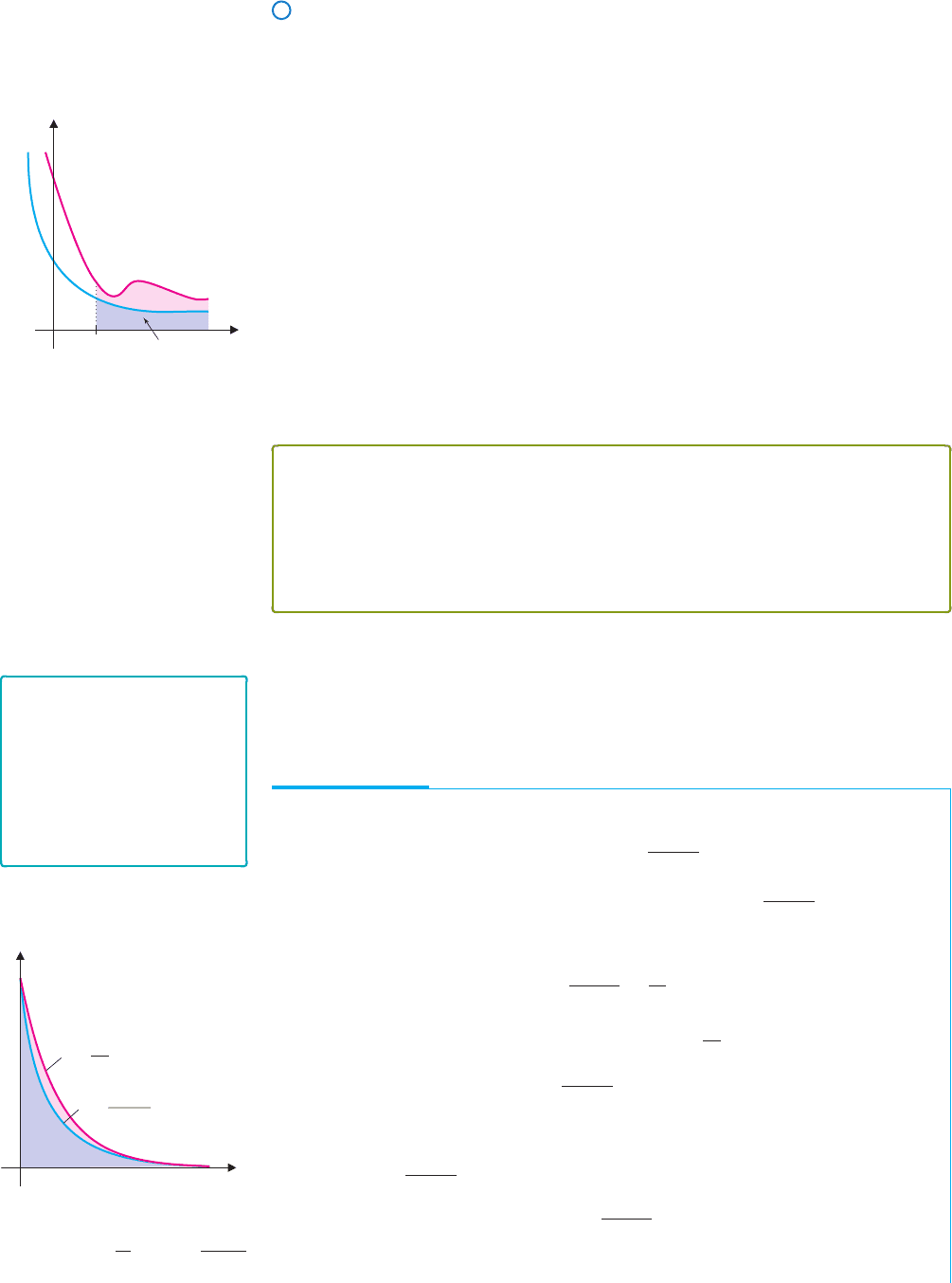
a
Smaller of
the two areas
y g(x)
y
f(x)
y
x
FIGURE 7.21
The Comparison Test
Given two functions f and g that are continuous on the interval [a, ∞), suppose that
0 ≤ f (x) ≤ g(x), for all x ≥ a.
We illustrate this situation in Figure 7.21. In this case,
∞
a
f (x) dx and
∞
a
g(x) dx
correspond to the areas under the respective curves. Notice that if
∞
a
g(x) dx (correspond-
ing to the larger area) converges, then this says that there is a finite area under the curve
y = g(x) on the interval [a, ∞). Since y = f (x) lies below y = g(x), there can be only a
finite area under the curve y = f (x), as well. Thus,
∞
a
f (x) dx converges also.
On the other hand, if
∞
a
f (x) dx (corresponding to the smaller area) diverges,the area
under the curve y = f (x) is infinite. Since y = g(x) lies above y = f (x), there must be
an infinite area under the curve y = g(x), also, so that
∞
a
g(x) dx diverges, as well. This
comparison of improper integrals based on the relative size of their integrands is called a
comparison test (one of several) and is spelled out in Theorem 7.1.
THEOREM 7.1 (Comparison Test)
Suppose that f and g are continuous on [a, ∞) and 0 ≤ f (x) ≤ g(x), for all
x ∈ [a, ∞).
(i) If
∞
a
g(x) dx converges, then
∞
a
f (x) dx converges, also.
(ii) If
∞
a
f (x) dx diverges, then
∞
a
g(x) dx diverges, also.
We omit the proof of Theorem 7.1, leaving it to stand on the intuitive argument already
made.
REMARK 7.1
We can state corresponding
comparison tests for improper
integrals of the form
a
−∞
f (x) dx, where f is
continuous on (−∞, a], as well
as for integrals that are
improper owing to a
discontinuity in the integrand.
The idea of the Comparison Test is to compare a given improper integral to another
improper integralwhose convergenceor divergenceis already known (or can be more easily
determined), as we illustrate in example 7.11.
EXAMPLE 7.11 Using the Comparison Test for an Improper Integral
Determine the convergence or divergence of
∞
0
1
x +e
x
dx.
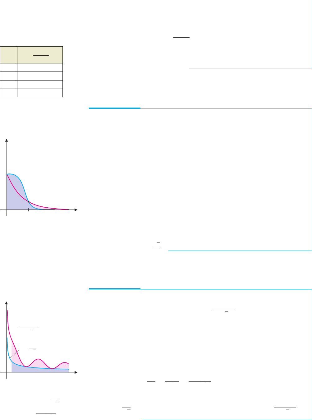
y
x
y
1
x e
x
y
1
e
x
FIGURE 7.22
Comparing y =
1
e
x
and y =
1
x + e
x
Solution First, note that you do not know an antiderivative for
1
x +e
x
and so, there is
no way to compute the improper integral directly. However, notice that for x ≥ 0,
0 ≤
1
x +e
x
≤
1
e
x
.
(See Figure 7.22.) It’s an easy exercise to show that
∞
0
1
e
x
dx converges (to 1). From
Theorem 7.1, it now follows that
∞
0
1
x +e
x
dx converges, also. While we know that
the integral is convergent, the Comparison Test does not help to find the value of the
integral. We can, however, use numerical integration (e.g., Simpson’s Rule) to
approximate
R
0
1
x +e
x
dx, for a sequence of values of R. The accompanying table
illustrates some approximate values of
R
0
1
x +e
x
dx, produced using the numerical
integration package built into our CAS. [If you use Simpson’s Rule for this, note that
you will need to increase the value of n (the number of subintervals in the partition) as
P1: OSO/OVY P2: OSO/OVY QC: OSO/OVY T1: OSO
MHDQ256-Ch07 MHDQ256-Smith-v1.cls December 23, 2010 21:26
LT (Late Transcendental)
CONFIRMING PAGES
7-55 SECTION 7.7
..
Improper Integrals 475
R increases.] Notice that as R gets larger and larger, the approximate values for the
corresponding integrals seem to be approaching 0.8063956, so we take this as an
approximate value for the improper integral.
∞
0
1
x +e
x
dx ≈ 0.8063956.
You should calculate approximate values for even larger values of R to convince
yourself that this estimate is accurate.
R
R
0
1
x e
x
dx
10 0.8063502
20 0.8063956
30 0.8063956
40 0.8063956
In example 7.12, we examine an integral that has important applications in probability
and statistics.
EXAMPLE 7.12 Using the Comparison Test for an Improper Integral
Determine the convergence or divergence of
∞
0
e
−x
2
dx.
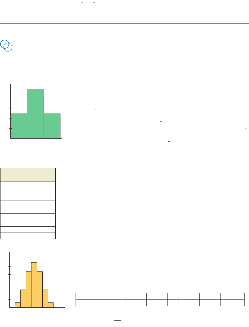
y
x
y e
−
x
2
1
y e
−
x
FIGURE 7.23
y = e
−x
2
and y = e
−x
Solution Once again, notice that you do not know an antiderivative for the integrand
e
−x
2
. However, observe that for x > 1, e
−x
2
< e
−x
. (See Figure 7.23.) We can rewrite
the integral as
∞
0
e
−x
2
dx =
1
0
e
−x
2
dx +
∞
1
e
−x
2
dx.
Since the first integral on the right-hand side is a proper definite integral, only the
second integral is improper. It’s an easy matter to show that
∞
1
e
−x
dx converges. By
the Comparison Test, it then follows that
∞
1
e
−x
2
dx also converges. We leave it as an
exercise to show that
∞
0
e
−x
2
dx =
1
0
e
−x
2
dx +
∞
1
e
−x
2
dx ≈ 0.8862269.
Using more advanced techniques of integration, it is possible to prove the surprising
result that
∞
0
e
−x
2
dx =
√
π
2
.
The Comparison Test can be used with equal ease to show that an improper integral is
divergent.
EXAMPLE 7.13 Using the Comparison Test: A Divergent Integral
Determine the convergence or divergence of
∞
1
2 + sin x
√
x
dx.
Solution As in examples 7.11 and 7.12, you do not know an antiderivative for the
integrand and so, your only hope for determining whether or not the integral converges
is to use a comparison. First, recall that
−1 ≤ sin x ≤ 1, for all x.
We then have that
0 <
1
√
x
=
2 − 1
√
x
≤
2 + sin x
√
x
, for 1 ≤ x < ∞.
(See Figure 7.24 for a graph of the two functions.) Recall that we showed in example
7.5 that
∞
1
1
√
x
dx diverges. The Comparison Test now tells us that
∞
1
2 + sin x
√
x
dx
must diverge, also.
y
x
y
2 sin x
兹x
y
1
兹x
FIGURE 7.24
Comparing y =
1
√
x
and
y =
2 + sin x
√
x

P1: OSO/OVY P2: OSO/OVY QC: OSO/OVY T1: OSO
MHDQ256-Ch07 MHDQ256-Smith-v1.cls December 23, 2010 21:26
LT (Late Transcendental)
CONFIRMING PAGES
476 CHAPTER 7
..
Integration Techniques 7-56
The big question, of course, is how to find an improper integral to compare to a
given integral. Look carefully at the integrand to see if it resembles any functions whose
antiderivativeyoumightknow(oratleasthaveahopeoffindingusingourvarioustechniques
ofintegration).Beyondthis,ourbestansweristhatthiscomeswithexperience.Comparisons
are typically done by the seat of your pants. We provideample exerciseson this topic to give
you some experience with finding appropriate comparisons. Look hard for comparisons and
don’t give up too easily.
BEYOND FORMULAS
It may seem that this section introduces an overwhelming number of new formulas
to memorize. Actually, all of the integrals introduced in this section follow a similar
pattern. In each case, we approximate the given integral by integrating over a different
interval.The exact value is then found by computing a limit as the approximate interval
approaches the desired interval. Answer the following for yourself. How do each of
the examples in this section fit this pattern?
EXERCISES 7.7
WRITING EXERCISES
1. For many students, our emphasis on working through the limit
process for an improper integral may seem unnecessarily care-
ful. Explain, using examples from this section, why it is im-
portant to have and use precise definitions.
2. Identify the following statement as true or false (meaning not
always true) and explain why: If the integrand f (x) →∞as
x → a
+
or as x → b
−
, then the area
b
a
f (x) dx is infinite;
that is,
b
a
f (x) dx diverges.
In exercises 1 and 2, determine whether or not the integral is
improper. If it is improper, explain why
1. (a)
2
0
x
−2/5
dx (b)
2
1
x
−2/5
dx (c)
2
0
x
2/5
dx
2. (a)
∞
0
x
2/5
dx (b)
2
−2
3
x
dx (c)
∞
2
3
x
dx
............................................................
In exercises 3–18, determine whether the integral converges or
diverges. Find the value of the integral if it converges.
3. (a)
1
0
x
−1/3
dx (b)
1
0
x
−4/3
dx
4. (a)
∞
1
x
−4/5
dx (b)
∞
1
x
−6/5
dx
5. (a)
1
0
1
√
1 − x
dx (b)
5
1
2
√
5 − x
dx
6. (a)
1
0
2
√
1 − x
2
dx (b)
1
0
2
x
√
1 − x
2
dx
7. (a)
∞
0
xe
x
dx (b)
∞
1
x
2
e
−2x
dx
8. (a)
1
−∞
x
2
e
3x
dx (b)
0
−∞
xe
−4x
dx
9. (a)
∞
−∞
1
x
2
dx (b)
∞
−∞
1
3
√
x
dx
10. (a)
∞
0
cos xdx (b)
∞
0
cos xe
−sinx
dx
11. (a)
1
0
ln xdx (b)
π
0
sec
2
xdx
12. (a)
π
0
cot xdx (b)
π/2
0
tan xdx
13. (a)
3
0
2
x
2
− 1
dx (b)
4
−4
2x
x
2
− 1
dx
14. (a)
π
0
x sec
2
xdx (b)
2
0
2
x
3
− 1
dx
15. (a)
∞
−∞
1
1 + x
2
dx (b)
∞
−∞
1
x
2
− 1
dx
16. (a)
2
0
x
x
2
− 1
dx (b)
∞
0
1
(x − 2)
2
dx
17. (a)
∞
0
1
√
xe
√
x
dx (b)
∞
0
tan xdx
18. (a)
∞
0
e
x
e
2x
+ 1
dx (b)
∞
0
x
√
x
2
+ 1
dx
............................................................

P1: OSO/OVY P2: OSO/OVY QC: OSO/OVY T1: OSO
MHDQ256-Ch07 MHDQ256-Smith-v1.cls December 23, 2010 21:26
LT (Late Transcendental)
CONFIRMING PAGES
7-57 SECTION 7.7
..
Improper Integrals 477
19. (a) Find all values of p for which
1
0
1
x
p
dx converges.
(b) Find all values of p for which
∞
1
1
x
p
dx converges.
(c) Show that
∞
−∞
x
p
dx diverges for every p.
20. (a) Find all values of r for which
∞
0
xe
rx
dx converges.
(b) Find all values of r for which
0
−∞
xe
rx
dx converges.
............................................................
In exercises 21–30, use a comparison to determine whether the
integral converges or diverges.
21.
∞
1
x
1 + x
3
dx 22.
∞
1
x
2
− 2
x
4
+ 3
dx
23.
∞
2
x
x
3/2
− 1
dx 24.
∞
1
2 + sec
2
x
x
dx
25.
∞
0
3
x + e
x
dx 26.
∞
1
e
−x
3
dx
27.
∞
0
sin
2
x
1 + e
x
dx 28.
∞
2
ln x
e
x
+ 1
dx
29.
∞
2
x
2
e
x
ln x
dx 30.
∞
1
e
x
2
+x+1
dx
............................................................
In exercises 31 and 32, use integration by parts and l’Hˆopital’s
Rule.
31.
1
0
x ln4xdx 32.
∞
0
xe
−2x
dx
............................................................
33. In this exercise, you will look at an interesting pair of calcula-
tions known as Gabriel’s horn. The horn is formed by taking
the curve y = 1/x for x ≥ 1 and revolving it about the x-axis.
Show that the volume is finite(i.e., the integral converges), but
that the surface area is infinite (i.e., the integral diverges). The
paradox is that this would seem to indicate that the horn could
be filled with a finite amount of paint but that the outside of
the horn could not be covered with any finite amount of paint.
34. Show that
∞
−∞
x
3
dx diverges but lim
R→∞
R
−R
x
3
dx = 0.
In exercises 35–38, determine whether the statement is true or
false (not always true).
35. If lim
x→∞
f (x) = 1, then
∞
0
f (x) dx diverges.
36. If lim
x→∞
f (x) = 0, then
∞
0
f (x) dx converges.
37. If lim
x→0
f (x) =∞, then
1
0
f (x) dx diverges.
38. If f (−x) =−f (x) for all x, then
∞
−∞
f (x) dx = 0.
............................................................
39. (a) Given that
∞
−∞
e
−x
2
dx =
√
π, evaluate
∞
−∞
e
−kx
2
dx
for k > 0.
(b) Given that
∞
−∞
e
−x
2
dx =
√
π, evaluate
∞
−∞
x
2
e
−kx
2
dx
for k > 0.
40. Given that
∞
0
sin x
x
dx =
π
2
, evaluate
∞
0
sin kx
x
dx for
(a) k > 0 (b) k < 0. Given that
∞
0
sin
2
x
x
2
dx =
π
2
, eval-
uate
∞
0
sin
2
kx
x
2
dx for (c) k > 0, (d) k < 0.
41. Noting that
x
x
5
+ 1
≈
1
x
4
for large values of x, explain why
you would expect
∞
0
x
x
5
+ 1
dx to converge. Use a compa-
rison test to prove that it does.
42. As in exercise 41, quickly conjecture whether the integral con-
verges or diverges.
(a)
∞
2
x
√
x
3
− 1
dx (b)
∞
2
x
√
x
5
− 1
dx
(c)
∞
2
x
√
x
5
+ x − 1
dx
43. Use the substitution u =
π
2
− x to show that
(a)
π/2
0
ln(sin x)dx =
π/2
0
ln(cos x)dx.Add
π/2
0
ln(sin x)dx
to both sides of this equation and simplify the right-hand side
with the identity sin2x = 2 sin x cos x. (b) Use this result to
show that 2
π/2
0
ln(sin x)dx =−
π
2
ln2 +
1
2
π
0
ln(sin x)dx.
(c) Show that
π
0
ln(sin x)dx = 2
π/2
0
ln(sin x)dx. (d) Use
parts (b) and (c) to evaluate
π/2
0
ln(sin x)dx.
44. Show that for any positive integer n,
1
0
(ln x)
n
dx equals n!if
n is even and −n!ifn is odd. [Hint: lim
x→0
+
x(ln x)
n
= 0.]
45. Explain why
π/2
0
1
1 + tan x
dx is an improper integral.
Assuming that it converges, explain why it is equal to
π/2
0
f (x) dx, where f (x) =
⎧
⎨
⎩
1
1 + tan x
if 0 ≤ x <
π
2
0ifx =
π
2
.
Similarly, find a function g(x) such that the improper
integral
π/2
0
tan x
1 + tan x
dx equals the proper integral
π/2
0
g(x)dx. Use the substitution u = x −
π
2
to show
that
π/2
0
1
1 + tan x
dx =
π/2
0
tan x
1 + tan x
dx. Adding the
first integral to both sides of the equation, evaluate
π/2
0
1
1 + tan x
dx.
46. Generalize exercise 45 to evaluate
π/2
0
1
1 + tan
k
x
dx for any
real number k.
47. Assuming that all integrals in this exercise converge,
use integration by parts to write
∞
−∞
x
4
e
−x
2
dx in terms
of
∞
−∞
x
2
e
−x
2
dx and then in terms of
∞
−∞
e
−x
2
dx =
√
π. By induction, show that
∞
−∞
x
2n
e
−x
2
dx =
(2n − 1)(2n − 3)···3 ·1
2
n
√
π, for any positive integer n.
48. Show that
∞
−∞
e
−ax
2
dx =
π
a
, for any positive constant
a = 0. Formally (that is, differentiate under the integral sign)
compute n derivatives with respect to a of this equation, set
a = 1 and compare the result to that of exercise 47.

P1: OSO/OVY P2: OSO/OVY QC: OSO/OVY T1: OSO
MHDQ256-Ch07 MHDQ256-Smith-v1.cls December 23, 2010 21:26
LT (Late Transcendental)
CONFIRMING PAGES
478 CHAPTER 7
..
Integration Techniques 7-58
APPLICATIONS
49. A function f (x) ≥ 0 is a probability density function (pdf) on
the interval [0, ∞)if
∞
0
f (x) dx = 1. Find the value of the
constant k to make each of the following pdf’s on the interval
[0, ∞).
(a) ke
−2x
(b) ke
−4x
(c) ke
−rx
, r > 0
50. Find the value of the constant k to make each of the following
pdf’s on the interval [0, ∞). (See exercise 49.)
(a) kxe
−2x
(b) kxe
−4x
(c) kxe
−rx
, r > 0
51. The mean μ (one measure of average) of a random variable
with pdf f (x) on the interval [0, ∞)isμ =
∞
0
xf(x) dx. Find
the mean of the exponential distribution f (x) = re
−rx
, r > 0.
52. Find the mean of a random variable with pdf f (x) = r
2
xe
−rx
.
53. Many probability questions involve conditional probabili-
ties. For example, if you know that a lightbulb has already
burned for 30 hours, what is the probability that it will last
at least 5 more hours? This is the “probability that x > 35
giventhat x > 30”andiswrittenas P(x > 35|x > 30).Ingen-
eral, for eventsA and B, P(A|B) =
P(A and B)
P(B)
, which in this
case reduces to P(x > 35|x > 30) =
P(x > 35)
P(x > 30)
. For the pdf
f (x) =
1
40
e
−x/40
(inhours),compute P(x > 35|x > 30).Also,
compute P(x > 40|x > 35) and P(x > 45|x > 40). (Hint:
P(x > 35) = 1 − P(x ≤ 35).)
54. Exercise 53 illustrates the“memoryless property” of exponen-
tial distributions. The probability that a lightbulb last m more
hours given that it has already lasted n hours depends only on
m and not on n. (a) Prove this for the pdf f (x) =
1
40
e
−x/40
.
(b) Show that any exponential pdf f (x) = ce
−cx
has the mem-
oryless property, for c > 0.
55. The Omega function is used for risk/reward analysis of fi-
nancial investments. Suppose that f (x) is a pdf on (−∞, ∞)
and gives the distribution of returns on an investment. (Then
b
a
f (x) dx is the probability that the investment returns
between $a and $b.) Let F(x) =
x
−∞
f (t)dt be the
cumulative distribution function for returns. Then
(r) =
∞
r
[1 − F(x)] dx
r
−∞
F(x) dx
is the Omega function for the
investment.
(a) Compute
1
(r) for the exponential distribution
f
1
(x) = 2e
−2x
, 0 ≤ x < ∞. Note that
1
(r) will be un-
defined (∞) for r ≤ 0.
(b) Compute
2
(r) for f
2
(x) = 1, 0 ≤ x ≤ 1.
(c) Show that the means of f
1
(x) and f
2
(x) are the same and
that (r) = 1 when r equals the mean.
(d) Even though the means are the same, investments with dis-
tributions f
1
(x)and f
2
(x)arenotequivalent.Usethegraphs
of f
1
(x) and f
2
(x) to explain why f
1
(x) corresponds to a
riskier investment than f
2
(x).
(e) Show that for some value c,
2
(r) >
1
(r) for r < c and
2
(r) <
1
(r) for r > c. In general, the larger (r) is,
the better the investment is. Explain this in terms of this
example.
56. The reliability function R(t) gives the probability that x > t.
For the pdf of a lightbulb, this is the probability that the bulb
lasts at least t hours. Compute R(t) for a general exponential
pdf f (x) = ce
−cx
.
57. The so-called Boltzmann integral
I(p) =
1
0
p(x)lnp(x) dx
is important in the mathematical field of information the-
ory. Here, p(x) is a pdf on the interval [0, 1]. Graph the pdf’s
p
1
(x) = 1 and
p
2
(x) =
4x if0 ≤ x ≤ 1/2
4 − 4x if1/2 ≤ x ≤ 1
and compute the integrals
1
0
p
1
(x)dx and
1
0
p
2
(x)dx to ver-
ify that they are pdf’s. Then compute the Boltzmann integrals
I(p
1
) and I (p
2
). Suppose that you are trying to determine the
valueof a quantitythat you know is between 0 and 1. If the pdf
forthisquantityis p
1
(x),thenallvaluesareequallylikely.What
would a pdf of p
2
(x) indicate? Noting that I (p
2
) > I (p
1
), ex-
plain why it is fair to say that the Boltzmann integral measures
the amount of information available. Given this interpretation,
sketch a pdf p
3
(x) that wouldhave a larger Boltzmann integral
than p
2
(x).
EXPLORATORY EXERCISES
1. The Laplace transform is an invaluable tool in many engi-
neering disciplines. As the name suggests, the transform turns
a function f (t) into a different function F(s). By definition,
the Laplace transform of the function f (t)is
F(s) =
∞
0
f (t)e
−st
dt.
To find the Laplace transform of f (t) = 1, compute
∞
0
(1)e
−st
dt =
∞
0
e
−st
dt.
Show that the integral equals 1/s, for s > 0. We write
L{1}=1/s. Show that
L{t}=
∞
0
te
−st
dt =
1
s
2
,
for s > 0. Compute L{t
2
}and L{t
3
}and conjecture the general
formula for L{t
n
}. Then, find L{e
at
} for s > a.
2. The gamma function is defined by (x) =
∞
0
t
x−1
e
−t
dt,if
the integral converges. For such a complicated-looking func-
tion, the gamma function has some surprising properties.
First, show that (1) = 1. Then use integration by parts and
l’Hˆopital’sRule toshowthat(n + 1) = n(n),foranyn > 0.
Use this property and mathematical induction to show that
(n + 1) = n!, for any positive integer n. (Notice that this
includes the value 0! = 1.) Numerically approximate
3
2
and
5
2
. Is it reasonable to define these as
1
2
! and
3
2
!,
P1: OSO/OVY P2: OSO/OVY QC: OSO/OVY T1: OSO
MHDQ256-Ch07 MHDQ256-Smith-v1.cls December 23, 2010 21:26
LT (Late Transcendental)
CONFIRMING PAGES
7-59 SECTION 7.8
..
Probability 479
respectively? In this sense, show that
1
2
! =
1
2
√
π. Finally,
for x < 1, the defining integral for (x) is improper in two
ways. Use a comparison test to show the convergence of
∞
1
t
x−1
e
−t
dt. This leaves
1
0
t
x−1
e
−t
dt. Determine the range
ofp-valuesforwhich
1
0
t
p
e
−t
dt convergesandthendetermine
the set of x’s for which (x) is defined.
7.8 PROBABILITY
The mathematical fields of probability and statistics focus on the analysis of random pro-
cesses.Inthissection,wegiveabriefintroductiontotheuseofcalculusinprobabilitytheory.
We begin with a simple example involving coin-tossing. Suppose that you toss two
coins, each of which has a 50% chance of coming up heads. Because of the randomness
involved, you cannot calculate exactly how many heads you will get on a given number of
tosses. But you can calculate the likelihood of each of the possible outcomes. If we denote
heads by H and tails by T, then the four possible outcomes from tossing two coins are HH,
HT, TH and TT. Each of these four outcomes is equally likely, so we can say that each has
probability
1
4
. This means that, on average, each of these events will occur in one-fourth of
your tries. Said a different way, the relative frequency with which each event occurs in a
large number of trials will be approximately
1
4
.
Note that based on our calculations above, the probability of getting two heads is
1
4
,
the probability of getting one head is
2
4
(since there are two ways for this to happen: HT and
TH) and the probability of getting zero heads is
1
4
. We often summarize such information
by displaying it in a histogram, a bar graph where the outcomes are listed on the horizontal
axis. (See Figure 7.25.)
012
0.1
0.2
0.3
0.4
0.5
FIGURE 7.25
Histogram for two-coin toss
If we instead toss eight coins, the probabilities for getting a given number of heads are
given in the accompanying table and the corresponding histogram is shown in Figure 7.26.
You should notice that the sum of all the probabilities is 1 (or 100%, since it’s certain that
one of the possible outcomes will occur on a given try). Thisis one of thedefining properties
of probability theory. Another basic property is called the addition principle: to compute
the probability of getting 6, 7 or 8 heads (or any other mutually exclusiveoutcomes), simply
add together the individual probabilities:
P(6, 7 or 8 heads) =
28
256
+
8
256
+
1
256
=
37
256
≈ 0.145.
Number
of Heads Probability
0 1/256
1 8/256
2 28/256
3 56/256
4 70/256
5 56/256
6 28/256
7 8/256
8 1/256
012345678
0.05
0.10
0.15
0.20
0.25
0.30
FIGURE 7.26
Histogram for eight-coin toss
A graphical interpretation of this calculation is very revealing. In the histogram in Fig-
ure 7.26, notice that each bar is a rectangle of width 1. Then the probability associated with
each bar equals the area of the rectangle. In graphical terms,
r
The total area in such a histogram is 1.
r
The probability of getting between 6 and 8 heads (inclusive) equals the sum of the
areas of the rectangles located between 6 and 8 (inclusive).
A more complicated question is to ask the probability that a randomly chosen person
will have a height of 5
9
or 5
10
. There is no easy theory we can use here to compute the
probabilities(sincenotallheightsareequallylikely).Inthiscase,weusethecorrespondence
between probability and relative frequency. If we collect information about the heights of
a large number of adults, we might find the following.
Height <64
64
65
66
67
68
69
70
71
72
73
>73
Number of people 23 32 61 94 133 153 155 134 96 62 31 26
Since the total number of people in the survey is 1000, the relative frequency of the
height 5
9
(69
)is
155
1000
= 0.155 and the relative frequency of the height 5
10
(70
)
is
134
1000
= 0.134. An estimate of the probability of being 5
9
or 5
10
is then
0.155 + 0.134 = 0.289. A histogram is shown in Figure 7.27.
P1: OSO/OVY P2: OSO/OVY QC: OSO/OVY T1: OSO
MHDQ256-Ch07 MHDQ256-Smith-v1.cls December 23, 2010 21:26
LT (Late Transcendental)
CONFIRMING PAGES
480 CHAPTER 7
..
Integration Techniques 7-60
0.02
0.04
0.06
0.08
0.10
0.12
0.14
0.16
64 64 65 66 67 68 69 70 71 72 73 73
FIGURE 7.27
Histogram for relative frequency of heights
To answer a more specific question, such as what the probability is that a randomly
chosen person is 5
8
1
2
or 5
9
, we would need to have our data broken down further, as in
the following partial table.
66
1
2
67
67
1
2
68
68
1
2
69
69
1
2
70
70
1
2
71
52 61 72 71 82 81 74 69 65 58
The probability that a person is 5
9
can be estimated by the relative frequency of
5
9
people in our survey, which is
81
1000
= 0.081. Similarly, the probability that a person
is 5
8
1
2
is approximately
82
1000
= 0.082. The probability of being 5
8
1
2
or 5
9
is then
approximately 0.082 +0.081 = 0.163. A histogram for this portion of the data is shown in
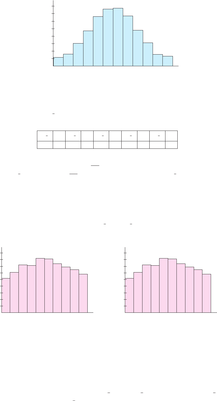
Figure 7.28a.
Notice that since each bar of the histogram now represents a half-inch range of height,
we can no longer interpret area in the histogram as the probability. We will modify the his-
togram to make the area connection clearer. In Figure 7.28b, we have labeled the horizontal
axis with the height in inches, while the vertical axis shows twice the relative frequency.
The bar at 69
has height 0.162 and width
1
2
. Its area,
1
2
(0.162) = 0.081, corresponds to the
relative frequency (or probability) of the height 5
9
.
67 68 69 70 71
0.09
0.08
0.07
0.06
0.05
0.04
0.03
0.02
0.01
67 68 69 70 71
0.18
0.16
0.14
0.12
0.10
0.08
0.06
0.04
0.02
FIGURE 7.28a
Histogram for relative frequency
of heights
FIGURE 7.28b
Histogram showing double the
relative frequency
Of course, we could continue subdividing the height intervals into smaller and smaller
pieces. Think of doing this while modifying the scale on the vertical axis so that the area of
each rectangle (length times width of interval) always gives the relative frequency (proba-
bility) of that height interval. For example, suppose that there are n height intervalsbetween
5
8
and5
9
.Let x represent height in inchesand f (x) equal the height of the histogram bar
for the interval containing x. Let x
1
= 68 +
1
n
, x
2
= 68 +
2
n
and so on, so that x
i
= 68 +
i
n
,
for 1 ≤ i ≤ n and let x =
1
n
. For a randomly selected person, the probability that their
P1: OSO/OVY P2: OSO/OVY QC: OSO/OVY T1: OSO
MHDQ256-Ch07 MHDQ256-Smith-v1.cls December 23, 2010 21:26
LT (Late Transcendental)
CONFIRMING PAGES
7-61 SECTION 7.8
..
Probability 481
height is between 5
8
and 5
9
is estimated by the sum of the areas of the corresponding
histogram rectangles, given by
P(68 ≤ x ≤ 69) ≈ f (x
1
)x + f (x
2
)x +···+ f (x
n
)x =
n
i=1
f (x
i
)x. (8.1)
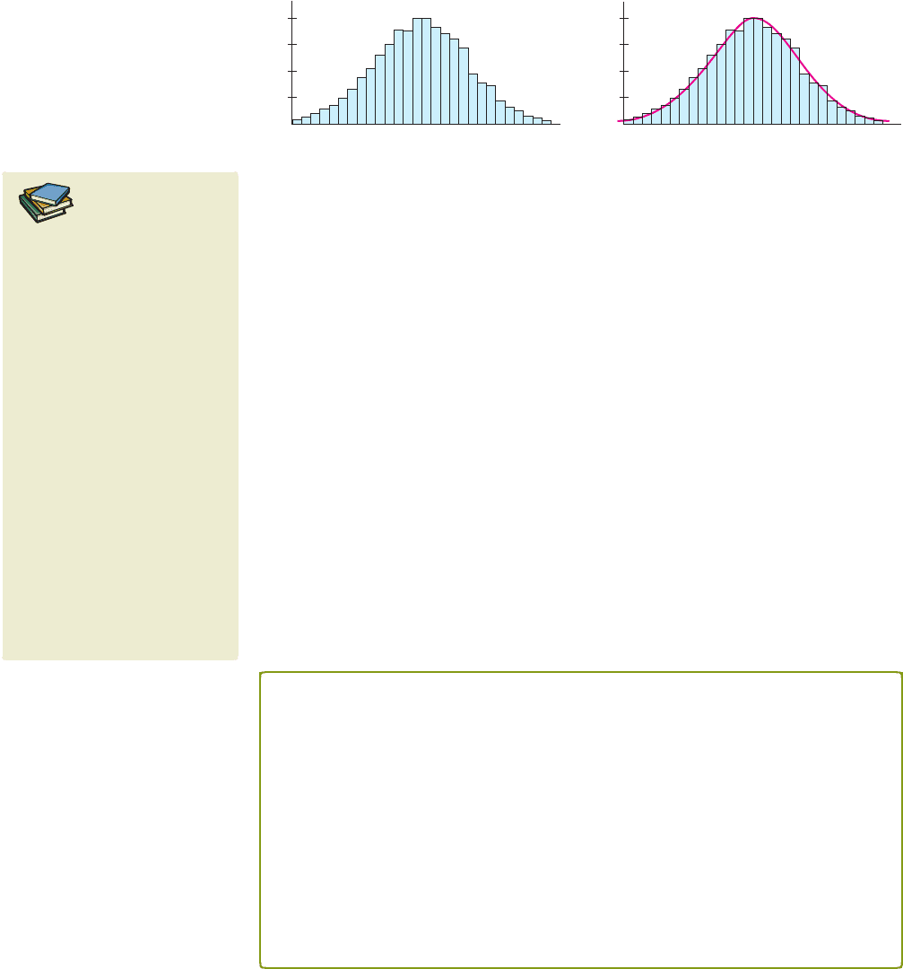
Observe that as n increases, the histogram of Figure 7.29 will “smooth out,” approaching a
curve like the one shown in Figure 7.30.
0.04
0.08
0.12
0.16
62 64 66 68 70 72 7463 65 67 69 71 73
0.04
0.08
0.12
0.16
62 64 66 68 70 72 7463 65 67 69 71 73
FIGURE 7.29
Histogram for heights
FIGURE 7.30
Probability density function and
histogram for heights
We call this limiting function f , the probability density function (pdf) for heights.
Notice that for any giveni = 1, 2,...,n, f (x
i
) does not give the probability that a person’s
height equals x
i
. Instead, for small values of x, the quantity f (x
i
)x is an approximation
of the probability that a randomly selected height is in the range [x
i−1
, x
i
].
Observe that as n →∞, the Riemann sum in (8.1) should approach an integral
b
a
f (x) dx. Here, the limits of integration are 68(5
8
) and 69(5
9
). We have
lim
n→∞
n
i=1
f (x
i
)x =
69
68
f (x) dx.
HISTORICAL
NOTES
Blaise Pascal (1623–1662)
A French mathematician and
physicist who teamed with Pierre
Fermat to begin the systematic
study of probability. (See The
Unfinished Game, by Keith Devlin,
for an account of this.) Pascal is
credited with numerous
inventions, including a wrist
watch, barometer, hydraulic
press, syringe and a variety of
calculating machines. He also
discovered what is now known as
Pascal’s Principle in hydrostatics.
(See section 5.6.) Pascal may well
have become one of the founders
of calculus, but poor health and
large periods of time devoted to
religious and philosophical
contemplation reduced his
mathematical output.
Notice that by adjusting the function values so that probability corresponds to area, we
have found a familiar and direct technique for computing probabilities. We now summarize
our discussion with some definitions. The preceding examples are of discrete probability
distributions (discrete since the quantity being measured can only assume values from a
certain finite set). For instance, in coin-tossing, the number of heads must be an integer. By
contrast, many distributions are continuous. That is, the quantity of interest (the random
variable) assumes values from a continuous range of numbers (an interval). For instance,
although height is normally rounded off to the nearest integer number of inches, a person’s
actual height can be any number.
For continuous distributions, the graph corresponding to a histogram is the graph of a
probability density function (pdf). We now give a precise definition of a pdf.
DEFINITION 8.1
Suppose that X is a random variable that may assume any value x with a ≤ x ≤ b.A
probability density function for X is a function f satisfying
(i) f (x) ≥0 for a ≤ x ≤ b.
Probability density functions are never negative.
and
(ii)
b
a
f (x) dx = 1. The total probability is 1.
The probability that the (observed) value of X falls between c and d is given by the
area under the graph of the pdf on that interval. That is,
P(c ≤ X ≤ d) =
d
c
f (x) dx. Probability corresponds to area under the curve.
To verify that a function defines a pdf for some (unknown) random variable, we must
show that it satisfies properties (i) and (ii) of Definition 8.1.
P1: OSO/OVY P2: OSO/OVY QC: OSO/OVY T1: OSO
MHDQ256-Ch07 MHDQ256-Smith-v1.cls December 23, 2010 21:26
LT (Late Transcendental)
CONFIRMING PAGES
482 CHAPTER 7
..
Integration Techniques 7-62
EXAMPLE 8.1 Verifying That a Function Is a pdf on an Interval
Show that f (x) = 3x
2
defines a pdf on the interval [0, 1] by verifying properties (i) and
(ii) of Definition 8.1.
Solution Clearly, f (x) ≥ 0. For property (ii), we integrate the pdf over its domain.
We have
1
0
3x
2
dx = x
3
1
0
= 1.
EXAMPLE 8.2 Using a pdf to Estimate Probabilities
Suppose that f (x) =
0.4
√
2π
e
−0.08(x−68)
2
is the probability density function for the
heights in inches of adult American males. Find the probability that a randomly selected
adult American male will be between 5
8
and 5
9
. Also, find the probability that a
randomly selected adult American male will be between 6
2
and 6
4
.
Solution To compute the probabilities, you first need to convert the specified heights
into inches. The probability of being between 68 and 69 inches tall is
P(68 ≤ X ≤ 69) =
69
68
0.4
√
2π
e
−0.08(x−68)
2
dx ≈ 0.15542.
Here, we approximated the value of the integral numerically. (You can use Simpson’s
Rule or the numerical integration method built into your calculator or CAS.) Similarly,
the probability of being between 74 and 76 inches is
P(74 ≤ X ≤ 76) =
76
74
0.4
√
2π
e
−0.08(x−68)
2
dx ≈ 0.00751,
where we have again approximated the value of the integral numerically.
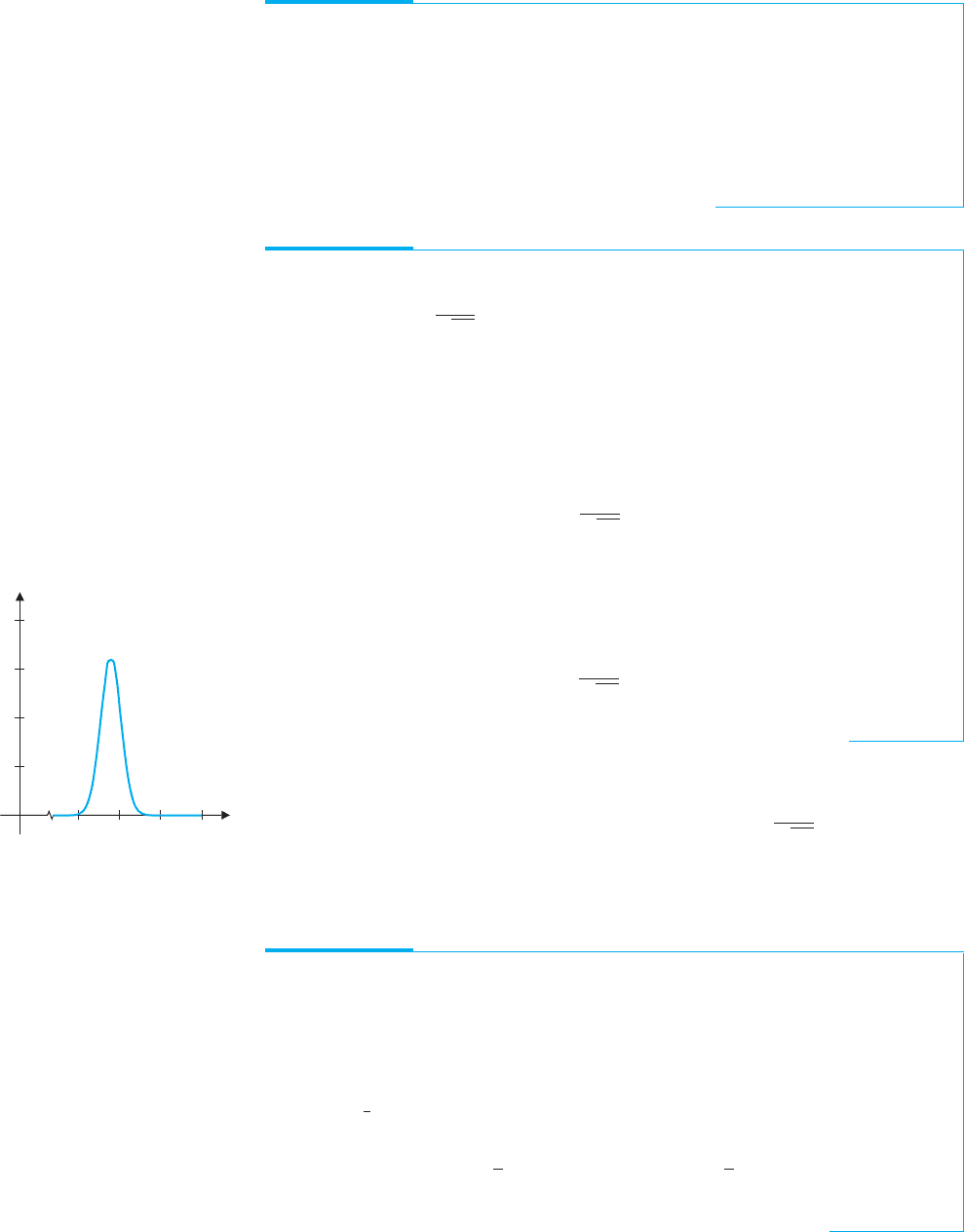
According to data in Gyles Brandreth’s Your Vital Statistics, the pdf for the heights of
adult males in the United States looks like the graph of f (x) =
0.4
√
2π
e
−0.08(x−68)
2
shown
in Figure 7.31 and used in example 8.2. You probably have seen bell-shaped curves like
this before. This distribution is referred to as a normal distribution. Besides the normal
distribution,thereare manyother probabilitydistributionsthatare importantinapplications.
y
60 70 80 90
0.05
0.10
0.15
0.20
x
FIGURE 7.31
Heights of adult males
EXAMPLE 8.3 Computing Probability with an Exponential pdf
Suppose that the lifetime in years of a certain brand of lightbulb is exponentially
distributed with pdf f (x) = 4e
−4x
. Find the probability that a given lightbulb lasts
3 months or less.
Solution First, since the random variable measures lifetime in years, convert
3 months to
1
4
year. The probability is then
P
0 ≤ X ≤
1
4
=
1/4
0
4e
−4x
dx = 4
−
1
4
e
−4x
1/4
0
=−e
−1
+ e
0
= 1 − e
−1
≈ 0.63212.
In some cases, there may be theoretical reasons for assuming that a pdf has a certain
form. In this event, the first task is to determine the values of any constants to achieve the
properties of a pdf.