Smith R., Minton R. Calculus
Подождите немного. Документ загружается.

P1: OSO/OVY P2: OSO/OVY QC: OSO/OVY T1: OSO
MHDQ256-Ch12 MHDQ256-Smith-v1.cls December 27, 2010 20:38
LT (Late Transcendental)
CONFIRMING PAGES
12-5 SECTION 12.1
..
Vector-Valued Functions 753
y
x
10
2
2
z
x
y
z
1
1
1
GRAPH A GRAPH B
y
x
z
10
10
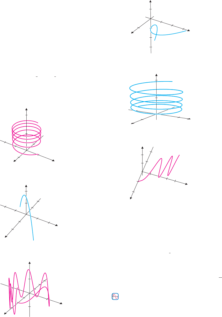
10
y
x
z
1
1
2
GRAPH C GRAPH D
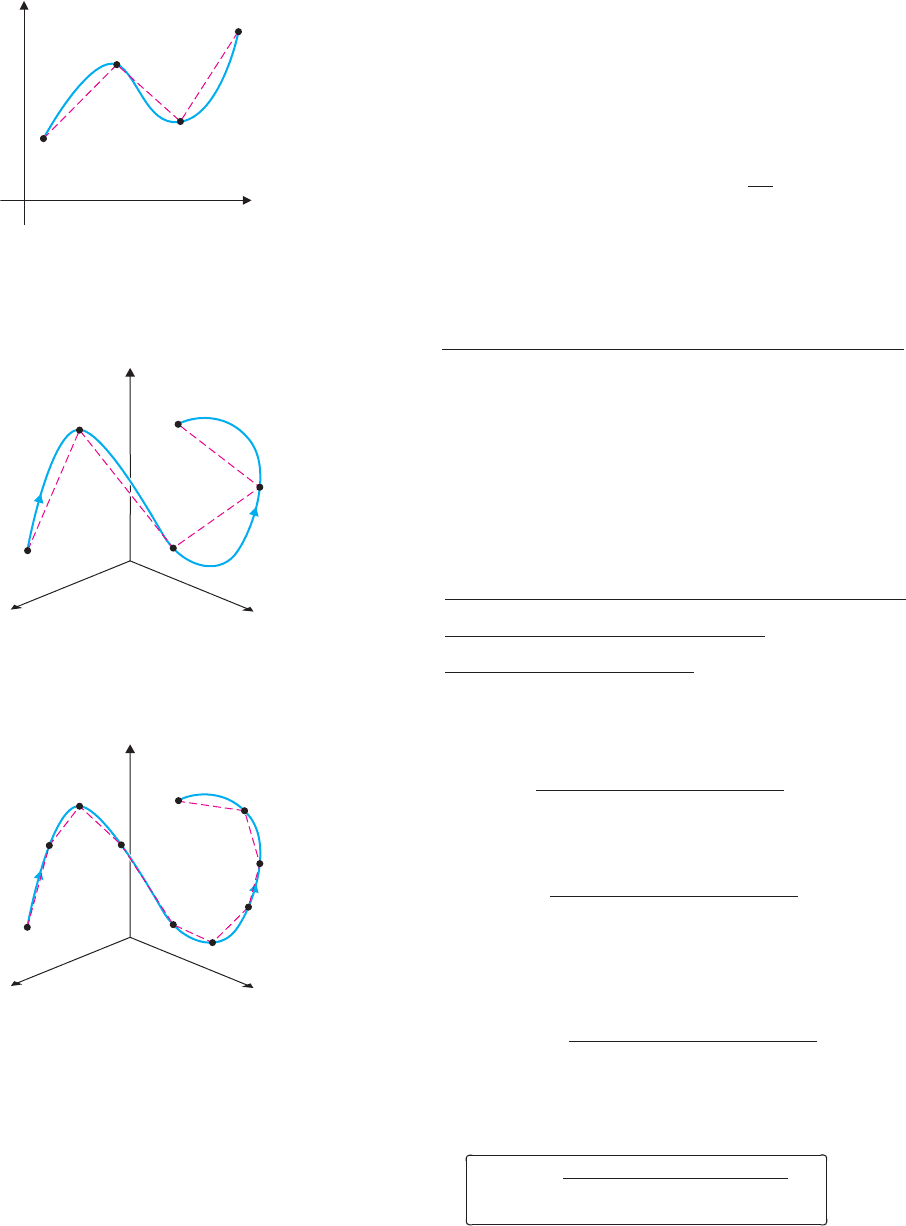
get closer together as you move to the right (as y →∞) and move very far apart as you
move to the left (as y →−∞). At first glance, you might expect the curve traced out by
f
2
(t) also to lie on a right circular cylinder, but look more closely. Here, we have
x = t cos t, y = t sin t and z = t, so that
x
2
+ y
2
= t
2
cos
2
t +t
2
sin
2
t = t
2
= z
2
.
This says that the curve lies on the surface defined by x
2
+ y
2
= z
2
(a right circular
cone with axis along the z-axis). Notice that only the curve shown in Graph C fits this
description. Next, notice that for f
3
(t), the y and z components are identical and so, the
curve must lie in the plane y = z. Replacing t by y,wehavex = 3sin 2t = 3sin 2y,a
sine curve lying in the plane y = z. Clearly, the curve in Graph D matches this
description. Although Graph A is the only curve remaining to match with f
4
(t), notice
that if the cosine and sine terms weren’t cubed, we’d simply have a helix, as in example
1.3. Since z = t, each point on the curve lies on the cylinder defined parametrically by
x = 5sin
3
t and y = 5cos
3
t. You need only look at the graph of the cross section of the
cylinder shown in Figure 12.6 (found by graphing the parametric equations x = 5sin
3
t
and y = 5cos
3
t in two dimensions) to decide that Graph A is the obvious choice.
y
x
5
55
5
FIGURE 12.6
A cross section of the cylinder
x = 5sin
3
t, y = 5cos
3
t
Arc Length in R
3
A natural question to ask about a curve is, “How long is it?” Note that the plane curve
tracedout exactlyonce by the endpoint of the vector-valued function r(t) =f (t), g(t), for
t ∈ [a, b] is the same as the curve defined parametrically by x = f (t), y = g(t). Recall
from section 10.3 that if f, f
, g and g
are all continuous for t ∈ [a, b], the arc length is
given by
s =
b
a
[ f
(t)]
2
+ [g
(t)]
2
dt. (1.3)
P1: OSO/OVY P2: OSO/OVY QC: OSO/OVY T1: OSO
MHDQ256-Ch12 MHDQ256-Smith-v1.cls December 27, 2010 20:38
LT (Late Transcendental)
CONFIRMING PAGES
754 CHAPTER 12
..
Vector-Valued Functions 12-6
We derived this by first breaking the curveinto small pieces (i.e., we partitioned the interval
[a, b]) and then approximating the length with the sum of the lengths of small line segments
connecting successive points. (See Figure 12.7a.) Finally, we made the approximation exact
by taking a limit as the number of points in the partition tended to infinity.
y
(f (a), g(a))
(f (b), g(b))
x
FIGURE 12.7a
Approximate arc length in R
2
y
x
z
O
C
FIGURE 12.7b
Approximate arc length in R
3
y
x
z
O
C
FIGURE 12.7c
Improved arc length approximation
Consider a space curve traced out by the endpoint of the vector-valued function
r(t) =f (t), g(t), h(t), where f, f
, g, g
, h and h
are all continuous for t ∈ [a, b] and
where the curve is traversed exactly once as t increases from a to b. As we did in the two-
dimensional case, we begin by partitioning the interval [a, b] into n subintervals of equal
size:a = t
0
< t
1
< ···< t
n
= b,wheret
i
− t
i−1
= t =
b−a
n
,foralli = 1, 2,...,n.Next,
for each i = 1, 2,...,n, we approximate the arc length s
i
of that portion of the curve join-
ing the points ( f (t
i−1
), g(t
i−1
), h(t
i−1
)) and ( f (t
i
), g(t
i
), h(t
i
)) by the straight-line distance
between the points. (See Figure 12.7b for an illustration of the case where n = 4.) From
the distance formula, we have
s
i
≈ d{( f (t
i−1
), g(t
i−1
), h(t
i−1
)), ( f (t
i
), g(t
i
), h(t
i
))}
=
[ f (t
i
) − f (t
i−1
)]
2
+ [g(t
i
) − g(t
i−1
)]
2
+ [h(t
i
) − h(t
i−1
)]
2
.
Applying the Mean Value Theorem three times (why can we do this?), we get
f (t
i
) − f (t
i−1
) = f
(c
i
)(t
i
− t
i−1
) = f
(c
i
)t,
g(t
i
) − g(t
i−1
) = g
(d
i
)(t
i
− t
i−1
) = g
(d
i
)t
and
h(t
i
) − h(t
i−1
) = h
(e
i
)(t
i
− t
i−1
) = h
(e
i
)t,
for some points c
i
, d
i
and e
i
in the interval (t
i−1
, t
i
). This gives us
s
i
≈
[ f (t
i
) − f (t
i−1
)]
2
+ [g(t
i
) − g(t
i−1
)]
2
+ [h(t
i
) − h(t
i−1
)]
2
=
[ f
(c
i
)t]
2
+ [g
(d
i
)t]
2
+ [h
(e
i
)t]
2
=
[ f
(c
i
)]
2
+ [g
(d
i
)]
2
+ [h
(e
i
)]
2
t.
Notice that if t is small, then all of c
i
, d
i
and e
i
are very close and we can make the further
approximation
s
i
≈
[ f
(c
i
)]
2
+ [g
(c
i
)]
2
+ [h
(c
i
)]
2
t,
for each i = 1, 2,...,n. The total arc length is then approximately
s ≈
n
i=1
[ f
(c
i
)]
2
+ [g
(c
i
)]
2
+ [h
(c
i
)]
2
t.
In Figure 12.7c, we illustrate this approximation for the case where n = 9. This suggests
that taking the limit as n →∞gives the exact arc length:
s = lim
n→∞
n
i=1
[ f
(c
i
)]
2
+ [g
(c
i
)]
2
+ [h
(c
i
)]
2
t,
provided the limit exists. You should recognize this as the definite integral
s =
b
a
[ f
(t)]
2
+ [g
(t)]
2
+ [h
(t)]
2
dt. (1.4)
Arc length
Observe that the arc length formulafor a plane curve (1.3) is a special case of (1.4). As with
other formulas for arc length, the integral in (1.4) can only rarely be computed exactly and
we must typically be satisfied with a numerical approximation. Example 1.6 illustrates one
of the very few arc lengths in R
3
that can be computed exactly.
P1: OSO/OVY P2: OSO/OVY QC: OSO/OVY T1: OSO
MHDQ256-Ch12 MHDQ256-Smith-v1.cls December 27, 2010 20:38
LT (Late Transcendental)
CONFIRMING PAGES
12-7 SECTION 12.1
..
Vector-Valued Functions 755
EXAMPLE 1.6 Computing Arc Length in R
3
Find the arc length of the curve traced out by the endpoint of the vector-valued function
r(t) =2t, lnt, t
2
, for 1 ≤ t ≤ e.
Solution First, notice that for x(t) = 2t, y(t) = lnt and z(t) = t
2
,wehavex
(t) = 2,
y
(t) =
1
t
and z
(t) = 2t, and the curve is traversed exactly once for 1 ≤ t ≤ e. (To see
why, observe that x = 2t is an increasing function.) From (1.4), we now have
s =
e
1
2
2
+
1
t
2
+ (2t)
2
dt =
e
1
4 +
1
t
2
+ 4t
2
dt
=
e
1
1 + 4t
2
+ 4t
4
t
2
dt =
e
1
(1 + 2t
2
)
2
t
2
dt
=
e
1
1 + 2t
2
t
dt =
e
1
1
t
+ 2t
dt
=
ln|t|+2
t
2
2
e
1
= (lne + e
2
) − (ln1 +1) = e
2
.
We show a graph of the curve for 1 ≤ t ≤ e in Figure 12.8.
y
x
z
FIGURE 12.8
The curve defined by
r(t) =2t, ln t, t
2
The arc length integral in example 1.7 is typical, in that we need a numerical
approximation.
EXAMPLE 1.7 Approximating Arc Length in R
3
Find the arc length of the curve traced out by the endpoint of the vector-valued function
r(t) =e
2t
, sin t, t, for 0 ≤ t ≤ 2.
Solution First, note that for x(t) = e
2t
, y(t) = sin t and z(t) = t, we have
x
(t) = 2e
2t
, y
(t) = cost and z
(t) = 1, and that the curve is traversed exactly once
for 0 ≤ t ≤ 2 (since x is an increasing function of t). From (1.4), we now have
s =
2
0
(2e
2t
)
2
+ (cos t)
2
+ 1
2
dt =
2
0
4e
4t
+ cos
2
t +1dt.
Since you don’t know how to evaluate this integral exactly (which is typically the case),
you can approximate the integral using Simpson’s Rule or the numerical integration
routine built into your calculator or computer algebra system, to find that the arc length
is approximately s ≈ 53.8.
Often,thecurveof interest is determined by the intersection of twosurfaces.Parametric
equations can give us simple representations of many such curves.
FIGURE 12.9a
Intersection of cone and plane
EXAMPLE 1.8 Finding Parametric Equations for an Intersection
of Surfaces
Find the arc length of the portion of the curve determined by the intersection of the cone
z =
x
2
+ y
2
and the plane y + z = 2 in the first octant.
Solution The cone and plane are shown in Figure 12.9a. From your knowledge of
conic sections, note that this curve could be a parabola or an ellipse. Parametric
equations for the curve must satisfy both z =
x
2
+ y
2
and y + z = 2. Eliminating z
by solving for it in each equation, we get
z =
x
2
+ y
2
= 2 − y.
Squaring both sides and gathering terms, we get
x
2
+ y
2
= (2 − y)
2
= 4 − 4y + y
2
or x
2
= 4 − 4y.
P1: OSO/OVY P2: OSO/OVY QC: OSO/OVY T1: OSO
MHDQ256-Ch12 MHDQ256-Smith-v1.cls December 27, 2010 20:38
LT (Late Transcendental)
CONFIRMING PAGES
756 CHAPTER 12
..
Vector-Valued Functions 12-8
Solving for y now gives us y = 1 −
x
2
4
,
which is clearly the equation of a parabola in two dimensions. To obtain the equation
for the three-dimensional parabola, let x be the parameter, which gives us the parametric
equations
x = t, y = 1 −
t
2
4
and z =
t
2
+ (1 −t
2
/4)
2
= 1 +
t
2
4
.
A graph is shown in Figure 12.9b. The portion of the parabola in the first octant must
have x ≥ 0 (so t ≥ 0), y ≥ 0 (so t
2
≤ 4) and z ≥ 0 (always true). This occurs if
0 ≤ t ≤ 2. The arc length is then
s =
2
0
1 + (−t/2)
2
+ (t/2)
2
dt =
√
2
2
ln
√
2 +
√
3
+
√
3 ≈ 2.54,
where we leave the details of the integration to you.
x
y
z
−5
−3.75
−2.5
−1.25
1.25
2.5
3.75
5
0
2.5
5
6
FIGURE 12.9b
Curve of intersection
BEYOND FORMULAS
If you think that examples 1.1 and 1.2 look very much like parametric equations
examples,you’re exactly right. The ideas presented there are not new; only the notation
and terminology are new. However, the vector notation lets us easilyextend these ideas
into three dimensions, where the graphs can be more complicated.
EXERCISES 12.1
WRITING EXERCISES
1. Discuss the differences, if any, between the curve traced
out by the terminal point of the vector-valued function
r(t) =f (t), g(t) and the curve defined parametrically by
x = f (t), y = g(t).
2. In example 1.3, describe the “shadow” of the helix in the
xy-plane (the shadow created by shining a light down from
the “top” of the z-axis). Equivalently, if the helix is collapsed
down into the xy-plane, describe the resulting curve. Compare
this curve to the ellipse defined parametrically by x = sint,
y =−3 cos t.
3. Discuss how you would compute the arc length of a curve
in four or more dimensions. Specifically, for the curve traced
out by the terminal point of the n-dimensional vector-valued
functionr(t) =f
1
(t), f
2
(t),..., f
n
(t)forn ≥ 4,state the arc
length formula and discuss how it relates to the n-dimensional
distance formula.
4. The helix in Figure 12.4a is shown from a standard view-
point (above the xy-plane, in between the x- and y-axes). De-
scribe what an observer at the point (0, 0, −1000) would see.
Also, describe what observers at the points (1000, 0, 0) and
(0, 1000, 0) would see.
Inexercises1–18,sketchthe curvetracedoutby the givenvector-
valued function by hand.
1. r(t) =t − 1, t
2
2. r(t) =t
2
− 1, 4t
3. r(t) = 2 costi +(sin t − 1)j4.r(t) = (sin t − 2)i + 4costj
5. r(t) =2 cos t, 2sint, 3 6. r(t) =cos2t, sin2t, 1
7. r(t) =t, t
2
+ 1, −1 8. r(t) =3, t, t
2
− 1
9. r(t) = ti + j +3t
2
k
10. r(t) = (t +2)i +(2t −1)j +(t +2)k
11. r(t) =4t −1, 2t +1, −6t
12. r(t) =−2t, 2t, 3 −t
13. r(t) = 3 costi +3 sin tj + tk
14. r(t) = 2 costi +sin tj + 3tk
15. r(t) =2 cos t, 2t, 3sin t
16. r(t) =−1, 2 cos t, 2 sin t
17. r(t) =t cos 2t, t sin 2t, 2t
18. r(t) =t cos t, 2t, t sin t
............................................................
In exercises 19–26, use graphing technology to sketch the curve
traced out by the given vector-valued function. Determine
whether the function is periodic; if so, name the period.
19. r(t) =cos 4t, sint, sin7t
20. r(t) =3 cos 2t, sin5t, cos t
21. r(t) = ti + tj + (2t
2
− 1)k
22. r(t) = (t
3
− t)i +t
2
j + (2t − 4)k
23. r(t) =tan t, sint
2
, cost
24. r(t) =sin t, −csct, cott
P1: OSO/OVY P2: OSO/OVY QC: OSO/OVY T1: OSO
MHDQ256-Ch12 MHDQ256-Smith-v1.cls December 27, 2010 20:38
LT (Late Transcendental)
CONFIRMING PAGES
12-9 SECTION 12.1
..
Vector-Valued Functions 757
25. (a) r(t) =2cost + sin2t, 2 sin t + cos 2t
(b) r(t) =2cos3t + sin5t, 2 sin 3t + cos 5t
(c) Howdoes the graph of 2 cosat +sinbt, 2sinat +cos bt
depend on a and b?
26. (a) r(t) =4cos4t − 6cost, 4 sin 4t − 6sint
(b) r(t) =4cos7t + 2cost, 4 sin 7t + 2 sin t
(c) How does the graph of
4cosat +b cos t, 4 sinat +b sint depend on a and b?
............................................................
27. In parts a–f, match the vector-valued function with its graph.
Give reasons for your choices.
(a) r(t) =cost
2
, t, t
(b) r(t) =cost, sin t, sin t
2
(c) r(t) =sin16
√
t, cos 16
√
t, t
(d) r(t) =sint
2
, cost
2
, t
(e) r(t) =t, t, 6 −4t
2
(f) r(t) =t
3
− t, 0.5t
2
, 2t − 4
y
x
1
1
z
GRAPH 1
y
x
1
1
4
z
GRAPH 2
y
x
1
1
1
z
GRAPH 3
y
x
1
2
4
4
4
8
12
z
GRAPH 4
y
x
1
1
z
GRAPH 5
y
x
2
1
1
2
2
3
4
4
z
GRAPH 6
28. Of the functions in exercise 27, which are periodic? Which are
bounded? Identify all components (x, y, z) that are bounded.
............................................................
In exercises 29–32, compute the arc length.
29. r(t) =t cos t, t sint,
1
3
(2t)
3/2
, 0 ≤ t ≤ 2π
30. r(t) =4t, 3 cost, 3sint, 0 ≤ t ≤ 3π
31. r(t) =4ln t, t
2
, 4t, 1 ≤ t ≤ 3
32. r(t) =tan
−1
t, ln(1 +t
2
), 2t − 2tan
−1
t, 0 ≤ t ≤
π
4
............................................................
In exercises 33–38, use a CAS to sketch the curve and estimate
its arc length.
33. r(t) =cos t, sint, cos2t, 0 ≤ t ≤ 2π
34. r(t) =cos t, sint, sint + cost, 0 ≤ t ≤ 2π
35. r(t) =cos π t, sinπt, cos16t, 0 ≤ t ≤ 2
P1: OSO/OVY P2: OSO/OVY QC: OSO/OVY T1: OSO
MHDQ256-Ch12 MHDQ256-Smith-v1.cls December 27, 2010 20:38
LT (Late Transcendental)
CONFIRMING PAGES
758 CHAPTER 12
..
Vector-Valued Functions 12-10
36. r(t) =cos π t, sinπt, cos16t, 0 ≤ t ≤ 4
37. r(t) =t, t
2
− 1, t
3
, 0 ≤ t ≤ 2
38. r(t) =t
2
+ 1, 2t, t
2
− 1, 0 ≤ t ≤ 2
............................................................
39. A spiral staircase makes two complete turns as it rises 10 feet
between floors. A handrail at the outside of the staircase is
located 3 feet from the center pole of the staircase. (a) Use
parametric equations for a helix to compute the length of the
handrail.(b)Imagine unrolling the staircasesothatthehandrail
is a line segment. Use theformula for the hypotenuseof a right
triangle to compute its length.
40. Find the arc length of the section of the helix traced out
by r(t) =cos t, sint, kt for 0 ≤ t ≤ 2π. As in exercise 39,
illustrate this as the hypotenuse of a right triangle.
In exercises 41–44, find parametric equations for the indicated
curve.If you have access to a graphing utility, graph the surfaces
and the resulting curve. Estimate its arc length.
41. The intersection of z =
x
2
+ y
2
and z = 2
42. The intersection of z =
x
2
+ y
2
and y + 2z = 2
43. The intersection of x
2
+ y
2
= 9 and y + z = 2
44. The intersection of y
2
+ z
2
= 9 and x = 2
............................................................
45. Show that the curve r(t) =2t, 4t
2
− 1, 8t
3
, 0 ≤ t ≤ 1, has
the same arc length as the curve in exercise 37.
46. Showthat the curve r(t) =t + 1, 2
√
t, t − 1, 0 ≤ t ≤ 4, has
the same arc length as the curve in exercise 38.
47. Compare the graphs of r(t) =t, t
2
, t
2
,
g(t) =cos t, cos
2
t, cos
2
t and h(t) =
√
t, t, t. Discuss the
similarities and the differences.
48. Comparethegraphsofr(t)=2t −1, t
2
, t, g(t)=2sint −1,
sin
2
t, sint and h(t) =2e
t
− 1, e
2t
, e
t
. Discuss the
similarities and the differences.
49. Show that the curve in exercise 33 lies on the hyperbolic
paraboloid z = x
2
− y
2
. Use a CAS to sketch both the surface
and the curve.
50. Show that the curve in exercise 34 lies onthe plane z = x + y.
Use a CAS to sketch both the plane and the curve.
51. (a) Use a graphing utility to sketch the graph of r(t) =
cost, cost, sin twith0 ≤ t ≤ 2π.Explain why the graph
should be the same with 0 ≤ t ≤ T, for any T ≥ 2π. Try
severallargerdomains(0 ≤ t ≤ 2π, 0 ≤ t ≤ 10π, 0 ≤ t ≤
50π, etc.) with your graphing utility. Eventually, the ellipse
should start looking thicker and for large enough domains
you will see a mess of jagged lines. Explain what has gone
wrong with the graphing utility.
(b) It may surprise you that this curve is not a circle. Show
that the shadows in the xz-plane and yz-plane are circles.
Show that the curve lies in the plane x = y. Sketch a graph
showing the plane x = y and a circular shadow in the yz-
plane. To draw a curve in the plane x = y with the circular
shadow, explain why the curve must be wider in the xy-
direction than in the z-direction. In other words, the curve
is not circular.
52. The graph of r(t) =cost, cos t,
√
2sintis a circle. To verify
this, start by showing that r(t)=
√
2, for all t.Then observe
that the curve lies in the plane x = y. Explain why this proves
that the graph is a (portion of a) circle.
EXPLORATORY EXERCISES
1. More insight into exercise 52 can begained by looking at basis
vectors. The circle traced out by r(t) =cos t, cost
√
2sint
lies in the plane x = y, which contains the vector
u =
1
√
2
1, 1, 0. The plane x = y also contains the vector
v =0, 0, 1. Show that any vector w in the plane x = y can
be written as w = c
1
u + c
2
v for some constants c
1
and c
2
.
Also, show that r(t) = (
√
2cost)u +(
√
2sint)v. Recall that
in two dimensions, a circle of radius r centered at the origin
can be written parametrically as (r cos t)i + (r sint)j. In gen-
eral, suppose that u and v are any orthogonal unit vectors. If
r(t) = (r cos t)u + (r sint)v, show that r(t) ·r(t) = r
2
.
2. Examine the graphs of several vector-valued functions of the
form r(t) =a cosct +b cos dt, a sinct + b sin dt, for con-
stants a, b, c and d. Determine the values of these constants
that produce graphs of different types. For example, starting
with the graph of 4cos4t − 6cost, 4 sin 4t − 6 sin t, change
c = 4toc = 3, c = 5, c = 2,etc.Conjecturearelationship be-
tween the number of loops and the difference between c and
d. Test this conjecture on other vector-valued functions. Re-
turning to 4 cos 4t − 6 cos t, 4sin4t − 6sint, change a = 4
to other values. Conjecture a relationship between the size of
the loops and the value of a.
12.2 THE CALCULUS OF VECTOR-VALUED FUNCTIONS
In this section, we begin to explore the calculus of vector-valued functions, beginning with
the notion of limit and progressing to continuity, derivatives and finally, integrals, just as
we did with scalar functions in Chapters 1, 2 and 4. We define everything in this section
in terms of vector-valued functions in three dimensions. The definitions can be interpreted
for vector-valued functions in two dimensions in the obvious way, by simply dropping the
third component everywhere.

P1: OSO/OVY P2: OSO/OVY QC: OSO/OVY T1: OSO
MHDQ256-Ch12 MHDQ256-Smith-v1.cls December 27, 2010 20:38
LT (Late Transcendental)
CONFIRMING PAGES
12-11 SECTION 12.2
..
The Calculus of Vector-Valued Functions 759
For a vector-valued function r(t) =f (t), g(t), h(t), when we write
lim
t→a
r(t) = u,
we mean that as t gets closer and closer to a, the vector r(t) is getting closer and closer to
the vector u.Foru =u
1
, u
2
, u
3
, this means that
lim
t→a
r(t) = lim
t→a
f (t), g(t), h(t)=u =u
1
, u
2
, u
3
.
Notice that for this to occur, we must have that f (t) is approaching u
1
, g(t) is approaching
u
2
and h(t) is approaching u
3
. In view of this, we make the following definition.
DEFINITION 2.1
For a vector-valued function r(t) =f (t), g(t), h(t), the limit of r(t)ast approaches
a is given by
lim
t→a
r(t) = lim
t→a
f (t), g(t), h(t)=
lim
t→a
f (t), lim
t→a
g(t), lim
t→a
h(t)
, (2.1)
provided all of the indicated limits exist. If any of the limits indicated on the
right-hand side of (2.1) fail to exist, then lim
t→a
r(t) does not exist.
In example 2.1, we see that calculating a limit of a vector-valued function simply
consists of calculating three separate limits of scalar functions.
EXAMPLE 2.1 Finding the Limit of a Vector-Valued Function
Find lim
t→0
t
2
+ 1, 5cost, sint.
Solution Here, each of the component functions is continuous (for all t) and so, we
can calculate their limits simply by substituting the value for t.Wehave
lim
t→0
t
2
+ 1, 5cost, sint=
lim
t→0
(t
2
+ 1), lim
t→0
(5cos t), lim
t→0
sint
=1, 5, 0.
EXAMPLE 2.2 A Limit That Does Not Exist
Find lim
t→0
e
2t
+ 5, t
2
+ 2t − 3, 1/t.
Solution Notice that the limit of the third component is lim
t→0
1
t
, which does not exist.
So, even though the limits of the first two components exist, the limit of the
vector-valued function does not exist.
Recall that for a scalar function f, we say that f is continuous at a if and only if
lim
t→a
f (t) = f (a).
That is, a scalar function is continuous at a point whenever the limit and the value of the
function are the same. We define the continuity of vector-valued functions in the same way.
DEFINITION 2.2
The vector-valued function r(t) =f (t), g(t), h(t) is continuous at t = a whenever
lim
t→a
r(t) = r(a)
(i.e., whenever the limit exists and equals the value of the vector-valued function).

P1: OSO/OVY P2: OSO/OVY QC: OSO/OVY T1: OSO
MHDQ256-Ch12 MHDQ256-Smith-v1.cls December 27, 2010 20:38
LT (Late Transcendental)
CONFIRMING PAGES
760 CHAPTER 12
..
Vector-Valued Functions 12-12
Notice that in terms of the components of r, this says that r(t) is continuous at t = a
whenever
lim
t→a
f (t), g(t), h(t)=
lim
t→a
f (t), lim
t→a
g(t), lim
t→a
h(t)
=f (a), g(a), h(a).
It then follows that r is continuous at t = a if and only if
lim
t→a
f (t) = f (a), lim
t→a
g(t) = g(a) and lim
t→a
h(t) = h(a).
Look carefully at what we have just said, and observe that we just proved the following
theorem.
THEOREM 2.1
A vector-valued function r(t) =f (t), g(t), h(t) is continuous at t = a if and only if
all of f, g and h are continuous at t = a.
Theorem 2.1 says that to determine where a vector-valued function is continuous, you
need only check the continuity of each component function (something you already know
how to do). We demonstrate this in examples 2.3 and 2.4.
EXAMPLE 2.3 Determining Where a Vector-Valued Function
Is Continuous
Determine the values of t for which the vector-valued function r(t) =e
5t
, ln(t + 1),
cost is continuous.
Solution From Theorem 2.1, r(t) will be continuous wherever all its components are
continuous. We have: e
5t
is continuous for all t, ln(t +1) is continuous for t > −1 and
cost is continuous for all t. So, r(t) is continuous for t > −1.
EXAMPLE 2.4 A Vector-Valued Function with Infinitely
Many Gaps in Its Domain
Determine the values of t for which the vector-valued function r(t) =
tant, |t +3|,
1
t−2
is continuous.
Solution First, note that tan t is continuous, except at t =
(2n + 1)π
2
, for
n = 0, ±1, ±2,...(i.e., except at odd multiples of
π
2
). The second component |t + 3| is
continuous for all t (although it’s not differentiable at t =−3). Finally, the third
component
1
t −2
is continuous except at t = 2. Since all three components must be
continuous in order for r(t) to be continuous, we have that r(t) is continuous, except at
t = 2 and t =
(2n + 1)π
2
, for n = 0, ±1, ±2,....
Recall that in Chapter 2, we defined the derivative of a scalar function f to be
f
(t) = lim
h→0
f (t + h) − f (t)
h
.
We replace h by t, to emphasize that t is an increment of the variable t. We then have
f
(t) = lim
t→0
f (t + t) − f (t)
t
.
P1: OSO/OVY P2: OSO/OVY QC: OSO/OVY T1: OSO
MHDQ256-Ch12 MHDQ256-Smith-v1.cls December 27, 2010 20:38
LT (Late Transcendental)
CONFIRMING PAGES
12-13 SECTION 12.2
..
The Calculus of Vector-Valued Functions 761
In Chapter 13, we’ll be defining partial derivatives of functions of more than one vari-
able, where we’ll use this type of notation to make it clear which variable is being
incremented.
We now define the derivative of a vector-valued function in the expected way.
DEFINITION 2.3
The derivative r
(t) of the vector-valued function r(t) is defined by
r
(t) = lim
t→0
r(t +t) − r(t)
t
, (2.2)
for any values of t for which the limit exists. When the limit exists for t = a,wesay
that r is differentiable at t = a.
Fortunately, you will not need to learn anynew differentiationrules, as the derivativeof
avector-valuedfunction is found directly from the derivativesof the individualcomponents,
as we see in Theorem 2.2.
THEOREM 2.2
Let r(t) =f (t), g(t), h(t) and suppose that the components f, g and h are all
differentiable for some value of t. Then r is also differentiable at that value of t and its
derivative is given by
r
(t) =f
(t), g
(t), h
(t). (2.3)
PROOF
From the definition of derivative of a vector-valued function (2.2), we have
r
(t) = lim
t→0
r(t +t) − r(t)
t
= lim
t→0
1
t
[ f (t + t), g(t + t), h(t + t)−f (t), g(t), h(t)]
= lim
t→0
1
t
f (t + t) − f (t), g(t + t) − g(t), h(t +t) − h(t),
= lim
t→0
f (t + t) − f (t)
t
,
g(t +t) − g(t)
t
,
h(t + t) −h(t)
t
=
lim
t→0
f (t + t) − f (t)
t
, lim
t→0
g(t +t) − g(t)
t
, lim
t→0
h(t + t) −h(t)
t
=f
(t), g
(t), h
(t),
where we have used the definition of limit of a vector-valued function (2.1) and where in the
last step we recognized the definition of the derivatives of each of the component functions
f, g and h.
P1: OSO/OVY P2: OSO/OVY QC: OSO/OVY T1: OSO
MHDQ256-Ch12 MHDQ256-Smith-v1.cls December 27, 2010 20:38
LT (Late Transcendental)
CONFIRMING PAGES
762 CHAPTER 12
..
Vector-Valued Functions 12-14
We illustrate this in example 2.5.
EXAMPLE 2.5 Finding the Derivative of a Vector-Valued Function
Find the derivative of r(t) =sin(t
2
), e
cost
, t lnt.
Solution Applying the chain rule to the first two components and the product rule to
the third, we have (for t > 0):
r
(t) =
d
dt
[sin(t
2
)],
d
dt
(e
cost
),
d
dt
(t lnt)
=
cos(t
2
)
d
dt
(t
2
), e
cost
d
dt
(cost),
d
dt
(t)lnt +t
d
dt
(lnt)
=
cos(t
2
)(2t), e
cost
(−sin t), (1)ln t + t
1
t
=2t cos(t
2
), −sinte
cost
, ln t + 1.
For the most part, to compute derivatives of vector-valued functions, we need only use
the already familiar rules for differentiation of scalar functions. There are several special
derivative rules, however, which we state in Theorem 2.3.
THEOREM 2.3
Suppose that r(t) and s(t) are differentiable vector-valued functions, f (t)isa
differentiable scalar function and c is any scalar constant. Then
(i)
d
dt
[r(t) +s(t)] = r
(t) +s
(t)
(ii)
d
dt
[c r(t)] = c r
(t)
(iii)
d
dt
[ f (t)r(t)] = f
(t)r(t) + f (t)r
(t)
(iv)
d
dt
[r(t) ·s(t)] = r
(t) ·s(t) + r(t) ·s
(t) and
(v)
d
dt
[r(t) ×s(t)] = r
(t) ×s(t) + r(t) ×s
(t).
Notice that parts (iii), (iv)and (v) are the product rules for the variouskinds of products
we can define. In each of these three cases, it’s important to recognize that these follow
the same pattern as the usual product rule for the derivative of the product of two scalar
functions.
PROOF
(i) For r(t) =f
1
(t), g
1
(t), h
1
(t) and s(t) =f
2
(t), g
2
(t), h
2
(t), we have from (2.3) and
the rules for vector addition that
d
dt
[r(t) +s(t)] =
d
dt
[ f
1
(t), g
1
(t), h
1
(t)+f
2
(t), g
2
(t), h
2
(t)]
=
d
dt
f
1
(t) + f
2
(t), g
1
(t) + g
2
(t), h
1
(t) + h
2
(t)
=f
1
(t) + f
2
(t), g
1
(t) + g
2
(t), h
1
(t) + h
2
(t)
=f
1
(t), g
1
(t), h
1
(t)+f
2
(t), g
2
(t), h
2
(t)
= r
(t) +s
(t).