Smith R., Minton R. Calculus
Подождите немного. Документ загружается.

P1: OSO/OVY P2: OSO/OVY QC: OSO/OVY T1: OSO
MHDQ256-Ch01 MHDQ256-Smith-v1.cls December 6, 2010 20:21
LT (Late Transcendental)
CONFIRMING PAGES
1-7 SECTION 1.2
..
The Concept of Limit 53
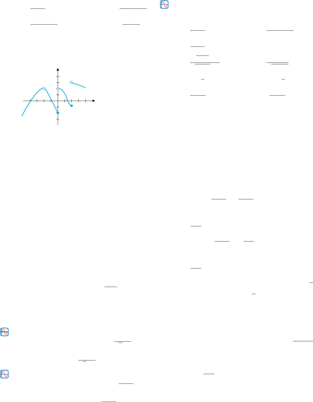
Notice that both functions are undefined at x = 2. So, what does this mean, beyond
saying that you cannot substitute 2 for x? We often find important clues about the behavior
of a function from a graph. (See Figures 1.7a and 1.7b.)
Notice that the graphs of these two functions look quite different in the vicinity of
x = 2. Although we can’t say anything about the value of these functions at x = 2 (since
this is outside the domain of both functions), we can examine their behavior in the vicinity
of this point. This is what limits will do for us.
EXAMPLE 2.1 Evaluating a Limit
Evaluate lim
x→2
x
2
− 4
x −2
.
Solution First, for f (x) =
x
2
− 4
x −2
, we compute some values of the function for x
close to 2, as in the following tables.
x f (x)
x
2
− 4
x − 2
1.9 3.9
1.99 3.99
1.999 3.999
1.9999 3.9999
x f (x)
x
2
− 4
x − 2
2.1 4.1
2.01 4.01
2.001 4.001
2.0001 4.0001
y
x
22
2
xx
4
f(x)
f(x)
FIGURE 1.7a
y =
x
2
− 4
x − 2
y
x
10510
10
5
5
10
x
x
f(x)
f(x)
FIGURE 1.7b
y =
x
2
− 5
x − 2
Notice that as you move down the first column of the first table, the x-values get
closer to 2, but are all less than 2. We use the notation x → 2
−
to indicate that x
approaches 2 from the left side. Notice that the table and the graph both suggest that as
x gets closer and closer to 2 (with x < 2), f (x) is getting closer and closer to 4. In view
of this, we say that the limit of f(x)asx approaches 2 from the left is 4, written
lim
x→2
−
f (x) = 4.
Similarly, we use the notation x → 2
+
to indicate that x approaches 2 from the
right side. We compute some of these values in the second table.
Again, the table and graph both suggest that as x gets closer and closer to 2 (with
x > 2), f (x) is getting closer and closer to 4. In view of this, we say that the limit of
f(x)asx approaches 2 from the right is 4, written
lim
x→2
+
f (x) = 4.
We call lim
x→2
−
f (x) and lim
x→2
+
f (x) one-sided limits. Since the two one-sided limits
of f (x) are the same, we summarize our results by saying that
lim
x→2
f (x) = 4.
The notion of limit as we have described it here is intended to communicate the
behavior of a function near some point of interest, but not actually at that point. We
finally observe that we can also determine this limit algebraically, as follows. Notice
that since the expression in the numerator of f (x) =
x
2
− 4
x −2
factors, we can write
lim
x→2
f (x) = lim
x→2
x
2
− 4
x −2
= lim
x→2
(x − 2)(x + 2)
x −2
Cancel the factors of (x −2).
= lim
x→2
(x + 2) = 4, As x approaches 2, (x + 2) approaches 4.
where we can cancel the factors of (x − 2) since in the limit as x → 2, x is close to 2,
but x = 2, so that x −2 = 0.
P1: OSO/OVY P2: OSO/OVY QC: OSO/OVY T1: OSO
MHDQ256-Ch01 MHDQ256-Smith-v1.cls December 6, 2010 20:21
LT (Late Transcendental)
CONFIRMING PAGES
54 CHAPTER 1
..
Limits and Continuity 1-8
EXAMPLE 2.2 A Limit That Does Not Exist
Evaluate lim
x→2
x
2
− 5
x −2
.
Solution As in example 2.1, we consider one-sided limits for g(x) =
x
2
− 5
x −2
,as
x → 2. Based on the graph in Figure 1.7b and the table of approximate function values
shown in the margin, observe that as x gets closer and closer to 2 (with x < 2), g(x)
increases without bound. Since there is no number that g(x) is approaching, we say that
the limit of g(x) as x approaches 2 from the left does not exist, written
lim
x→2
−
g(x) does not exist.
x g(x)
x
2
− 5
x − 2
1.9 13.9
1.99 103.99
1.999 1003.999
1.9999 10,003.9999
x g(x)
x
2
− 5
x − 2
2.1 −5.9
2.01 −95.99
2.001 −995.999
2.0001 −9995.9999
Similarly, the graph and the table of function values for x > 2 (shown in the
margin) suggest that g(x) decreases without bound as x approaches 2 from the right.
Since there is no number that g(x) is approaching, we say that
lim
x→2
+
g(x) does not exist.
Finally, since there is no common value for the one-sided limits of g(x) (in fact,
neither limit exists), we say that
lim
x→2
g(x) does not exist.
Before moving on, we should summarize what we have said about limits.
A limit exists if and only if both corresponding one-sided limits exist and are equal.
That is,
lim
x→a
f (x) = L, for some number L, if and only if lim
x→a
−
f (x) = lim
x→a
+
f (x) = L.
In other words, we say that lim
x→a
f (x) = L if we can make f (x) as close as we might like to
L, by making x sufficiently close to a (on either side of a), but not equal to a.
Note that we can think about limits from a purely graphical viewpoint, as in
example 2.3.
y
x
1 2
2
1
1
2
2 1
FIGURE 1.8
y = f (x)
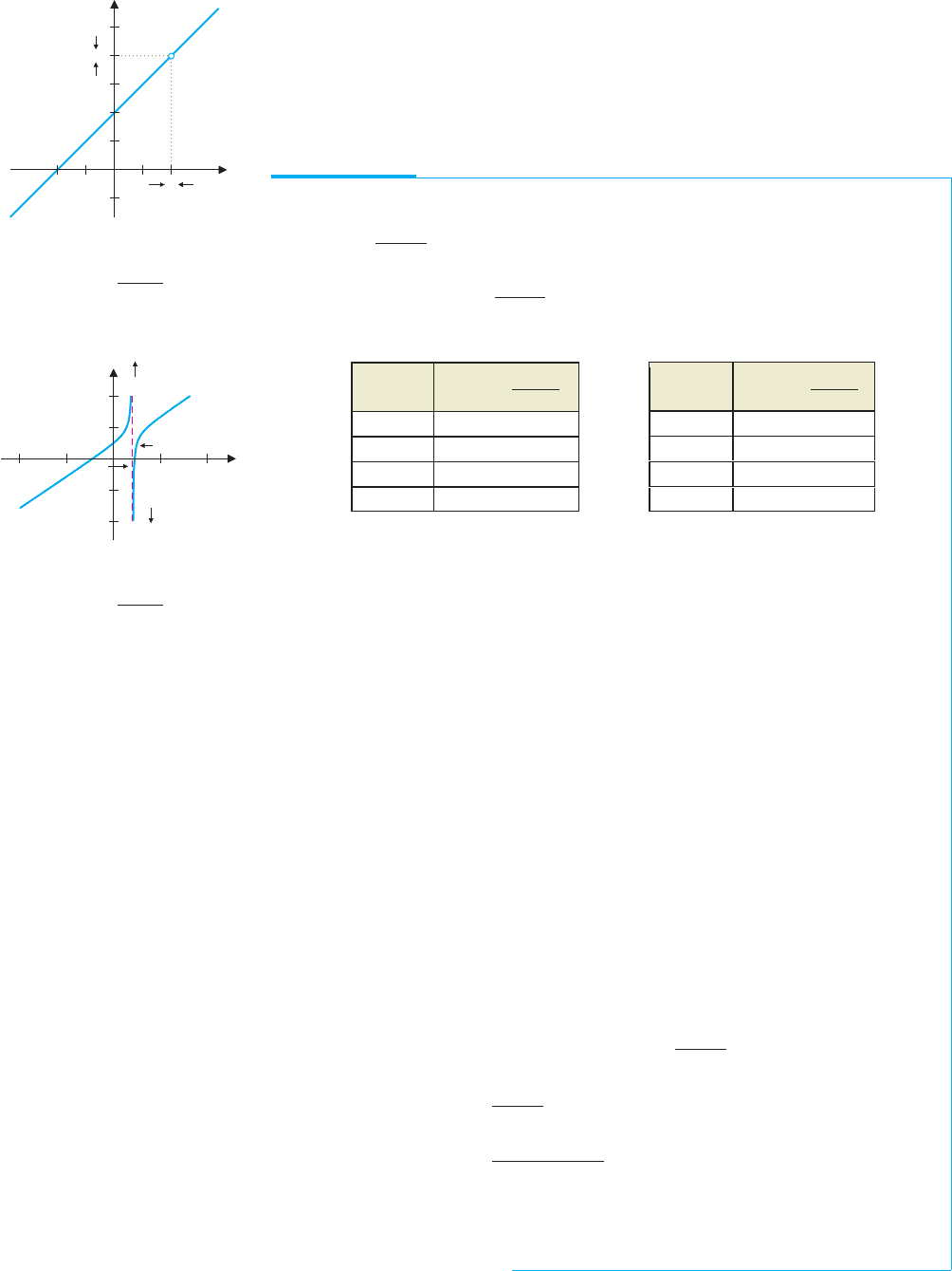
EXAMPLE 2.3 Determining Limits Graphically
Use the graph in Figure 1.8 to determine lim
x→1
−
f (x), lim
x→1
+
f (x), lim
x→1
f (x) and lim
x→−1
f (x).
Solution For lim
x→1
−
f (x), we consider the y-values as x gets closer to 1, with x < 1.
That is, we follow the graph toward x = 1 from the left (x < 1). Observe that the graph
dead-ends into the open circle at the point (1, 2). Therefore, we say that lim
x→1
−
f (x) = 2.
For lim
x→1
+
f (x), we follow the graph toward x = 1 from the right (x > 1). In this case,
the graph dead-ends into the solid circle located at the point (1, −1). For this reason, we
say that lim
x→1
+
f (x) =−1. Because lim
x→1
−
f (x) = lim
x→1
+
f (x), we say that lim
x→1
f (x) does
not exist. Finally, we have that lim
x→−1
f (x) = 1, since the graph approaches a y-value of
1asx approaches −1 both from the left and from the right.
P1: OSO/OVY P2: OSO/OVY QC: OSO/OVY T1: OSO
MHDQ256-Ch01 MHDQ256-Smith-v1.cls December 6, 2010 20:21
LT (Late Transcendental)
CONFIRMING PAGES
1-9 SECTION 1.2
..
The Concept of Limit 55
y
x
2
Q
3
xx
3
3
f(x)
f(x)
FIGURE 1.9
lim
x→−3
3x + 9
x
2
− 9
=−
1
2
x
3x 9
x
2
− 9
−3.1 −0.491803
−3.01 −0.499168
−3.001 −0.499917
−3.0001 −0.499992
x
3x 9
x
2
− 9
−2.9 −0.508475
−2.99 −0.500835
−2.999 −0.500083
−2.9999 −0.500008
EXAMPLE 2.4 A Limit Where Two Factors Cancel
Evaluate lim
x→−3
3x + 9
x
2
− 9
.
Solution We examine a graph (see Figure 1.9) and compute some function values for
x near −3. Based on this numerical and graphical evidence, it’s reasonable to conjecture
that
lim
x→−3
−
3x + 9
x
2
− 9
= lim
x→−3
−
3x + 9
x
2
− 9
=−
1
2
.
Further, note that
lim
x→−3
−
3x + 9
x
2
− 9
= lim
x→−3
−
3(x + 3)
(x + 3)(x − 3)
Cancel factors of (x +3).
= lim
x→−3
−
3
x −3
=−
1
2
,
since (x − 3) →−6asx →−3. Again, the cancellation of the factors of (x +3) is
valid since in the limit as x →−3, x is close to −3, but x =−3, so that x + 3 = 0.
Likewise,
lim
x→−3
+
3x + 9
x
2
− 9
=−
1
2
.
Finally, since the function approaches the same value as x →−3 both from the
right and from the left (i.e., the one-sided limits are equal), we write
lim
x→−3
3x + 9
x
2
− 9
=−
1
2
.
In example 2.4, the limit exists because both one-sided limits exist and are equal. In
example 2.5, neither one-sided limit exists.
y
x
x
x
3
30
30
f(x)
f(x)
FIGURE 1.10
y =
3x + 9
x
2
− 9
x
3x 9
x
2
− 9
3.1 30
3.01 300
3.001 3000
3.0001 30,000
x
3x 9
x
2
− 9
2.9 −30
2.99 −300
2.999 −3000
2.9999 −30,000
EXAMPLE 2.5 A Limit That Does Not Exist
Determine whether lim
x→3
3x + 9
x
2
− 9
exists.
Solution We first draw a graph (see Figure 1.10) and compute some function values
for x close to 3.
Based on this numerical and graphical evidence, it appears that, as x → 3
+
,
3x + 9
x
2
− 9
is increasing without bound. Thus,
lim
x→3
+
3x + 9
x
2
− 9
does not exist.
Similarly, from the graph and the table of values for x < 3, we can say that
lim
x→3
−
3x + 9
x
2
− 9
does not exist.
Since neither one-sided limit exists, we say
lim
x→3
3x + 9
x
2
− 9
does not exist.
Here, we considered both one-sided limits for the sake of completeness. Of course, you
should keep in mind that if either one-sided limit fails to exist, then the limit does not
exist.
Many limits cannot be resolved using algebraic methods. In these cases, we can
approximate the limit using graphical and numerical evidence, as we see in example 2.6.
P1: OSO/OVY P2: OSO/OVY QC: OSO/OVY T1: OSO
MHDQ256-Ch01 MHDQ256-Smith-v1.cls December 6, 2010 20:21
LT (Late Transcendental)
CONFIRMING PAGES
56 CHAPTER 1
..
Limits and Continuity 1-10
EXAMPLE 2.6 Approximating the Value of a Limit
Evaluate lim
x→0
sin x
x
.
Solution Unlike some of the limits considered previously, there is no algebra that will
simplify this expression. However, we can still draw a graph (see Figure 1.11) and
compute some function values.
y
x
xx
424 2
1
f(x)
FIGURE 1.11
lim
x→0
sin x
x
= 1
x
sin x
x
0.1 0.998334
0.01 0.999983
0.001 0.99999983
0.0001 0.9999999983
0.00001 0.999999999983
x
sin x
x
−0.1 0.998334
−0.01 0.999983
−0.001 0.99999983
−0.0001 0.9999999983
−0.00001 0.999999999983
The graph and the tables of values lead us to the conjectures:
lim
x→0
+
sin x
x
= 1 and lim
x→0
−
sin x
x
= 1,
from which we conjecture that
lim
x→0
sin x
x
= 1.
In Chapter 2, we examine these limits with greater care (and prove that these
conjectures are correct).
REMARK 2.1
Computer or calculator computation of limits is unreliable. We use graphs and tables
of values only as (strong) evidence pointing to what a plausible answer might be. To
be certain, we need to obtain careful verification of our conjectures. We explore this
in sections 1.3–1.7.
y
x
44
1
1
FIGURE 1.12a
y =
x
|x|
y
x
22
1
1
x
x
f(x)
f(x)
FIGURE 1.12b
lim
x→0
x
|x|
does not exist.
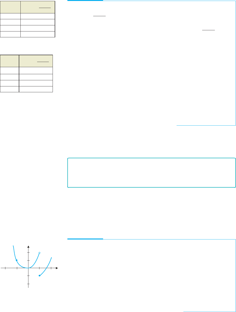
EXAMPLE 2.7 A Case Where One-Sided Limits Disagree
Evaluate lim
x→0
x
|x|
.
Solution The computer-generated graph shown in Figure 1.12a is incomplete. Since
x
|x|
is undefined at x = 0, there is no point at x = 0. The graph in Figure 1.12b
correctly shows open circles at the intersections of the two halves of the graph with the
y-axis. We also have
lim
x→0
+
x
|x|
= lim
x→0
+
x
x
Since |x|=x, when x > 0.
= lim
x→0
+
1
= 1
and lim
x→0
−
x
|x|
= lim
x→0
−
x
−x
Since |x|=−x, when x < 0.
= lim
x→0
−
−1
=−1.
It now follows that lim
x→0
x
|x|
does not exist,
since the one-sided limits are not the same. You should also keep in mind that this
observation is entirely consistent with what we see in the graph.

P1: OSO/OVY P2: OSO/OVY QC: OSO/OVY T1: OSO
MHDQ256-Ch01 MHDQ256-Smith-v1.cls December 6, 2010 20:21
LT (Late Transcendental)
CONFIRMING PAGES
1-11 SECTION 1.2
..
The Concept of Limit 57
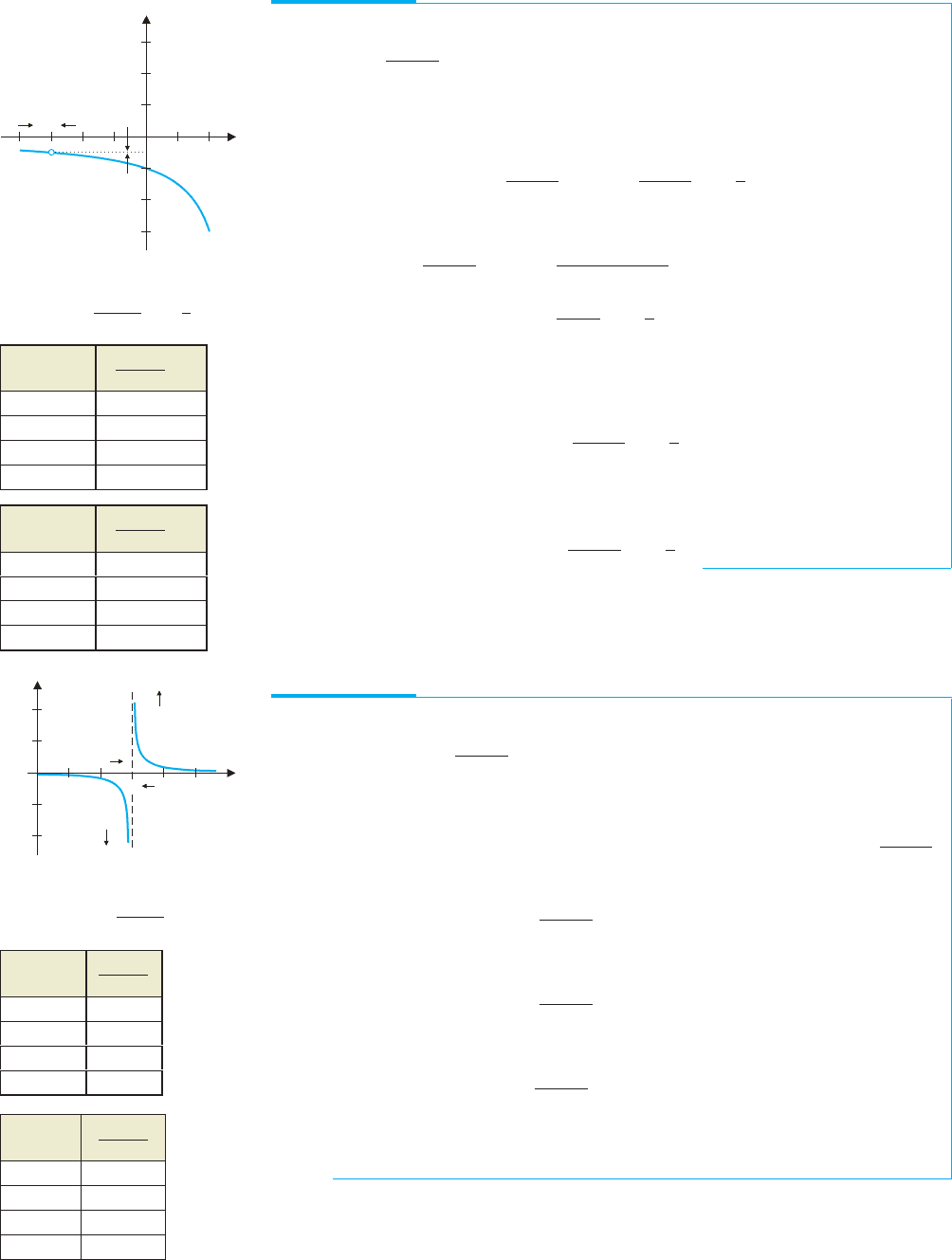
EXAMPLE 2.8 A Limit Describing the Movement of a Baseball Pitch
The knuckleball is one of the most exotic pitches in baseball. Batters describe the ball as
unpredictably moving left, right, up and down. For a typical knuckleball speed of
60 mph, the left/right position of the ball (in feet) as it crosses the plate is given by
f (ω) =
1.7
ω
−
5
8ω
2
sin(2.72ω)
(derived from experimental data in Watts and Bahill’s book Keeping Your Eye on the
Ball), where ω is the rotational speed of the ball in radians per second and where
f (ω) = 0 corresponds to the middle of home plate. Folk wisdom among baseball
pitchers has it that the less spin on the ball, the better the pitch. To investigate this
theory, we consider the limit of f (ω)asω → 0
+
. As always, we look at a graph (see
Figure 1.13) and generate a table of function values. The graphical and numerical
evidence suggests that lim
ω→0
+
f (ω) = 0.
y
v
0.5
1.0
1.5
210864
FIGURE 1.13
y =
1.7
ω
−
5
8ω
2
sin(2.72ω)
ω f (ω)
10 0.1645
1 1.4442
0.1 0.2088
0.01 0.021
0.001 0.0021
0.0001 0.0002
The limit indicates that a knuckleball with absolutely no spin doesn’t move at
all (and therefore would be easy to hit). According to Watts and Bahill, a very slow
rotation rate of about 1 to 3 radians per second produces the best pitch (i.e., the most
movement). Take another look at Figure 1.13 to convince yourself that this makes
sense.
EXERCISES 1.2
WRITING EXERCISES
1. Suppose your professor says, “The limit is a prediction of what
f (a)willbe.”Critiquethisstatement.Whatdoesitmean?Does
itprovideimportantinsight?Isthereanythingmisleadingabout
it? Replace the phrase in italics with your own best description
of what the limit is.
2. In example 2.6, we conjecture that lim
x→0
sin x
x
= 1. Discuss the
strength of the evidence for this conjecture. If it were true that
sin x
x
= 0.998 for x = 0.00001, how much would our case
be weakened? Can numerical and graphical evidence ever be
completely conclusive?
3. We have observed that lim
x→a
f (x) does not depend on the actual
value of f (a), or even on whether f (a) exists. In principle,
functions such as f (x) =
x
2
if x = 2
13 if x = 2
are as “normal” as
functions such as g(x) = x
2
. With this in mind, explain why
it is important that the limit concept is independent of how (or
whether) f (a) is defined.
4. The most common limit encountered in everyday life is the
speed limit. Describe how this type of limit is very different
from the limits discussed in this section.
In exercises 1–6, use numerical and graphical evidence to con-
jecture values for each limit. If possible, use factoring to verify
your conjecture.
1. lim
x→1
x
2
− 1
x − 1
2. lim
x→−1
x
2
+ x
x
2
− x − 2
P1: OSO/OVY P2: OSO/OVY QC: OSO/OVY T1: OSO
MHDQ256-Ch01 MHDQ256-Smith-v1.cls December 6, 2010 20:21
LT (Late Transcendental)
CONFIRMING PAGES
58 CHAPTER 1
..
Limits and Continuity 1-12
3. lim
x→2
x − 2
x
2
− 4
4. lim
x→1
(x − 1)
2
x
2
+ 2x − 3
5. lim
x→3
3x − 9
x
2
− 5x + 6
6. lim
x→−2
2 + x
x
2
+ 2x
............................................................
In exercises 7 and 8, identify each limit or state that it does not
exist.
y
x
42
2
2
4
4
7.
(a) lim
x→0
−
f (x) (b) lim
x→0
+
f (x) (c) lim
x→0
f (x)
(d) lim
x→−2
−
f (x) (e) lim
x→−2
+
f (x) (f) lim
x→−2
f (x)
(g) lim
x→−1
f (x) (h) lim
x→1
−
f (x)
8.
(a) lim
x→1
−
f (x) (b) lim
x→1
+
f (x) (c) lim
x→1
f (x)
(d) lim
x→2
−
f (x) (e) lim
x→2
+
f (x) (f) lim
x→2
f (x)
(g) lim
x→3
−
f (x) (h) lim
x→−3
f (x)
............................................................
9. Sketch the graph of f (x) =
2x if x < 2
x
2
if x ≥ 2
and identify
each limit.
(a) lim
x→2
−
f (x) (b) lim
x→2
+
f (x) (c) lim
x→2
f (x)
(d) lim
x→1
f (x) (e) lim
x→3
f (x)
10. Sketch the graph of f (x) =
⎧
⎪
⎨
⎪
⎩
x
3
− 1ifx < 0
0ifx = 0
√
x + 1 − 2ifx > 0
and identify each limit.
(a) lim
x→0
−
f (x) (b) lim
x→0
+
f (x) (c) lim
x→0
f (x)
(d) lim
x→−1
f (x) (e) lim
x→1
−
f (x)
11. Evaluate f (1.5), f (1.1), f (1.01) and f (1.001), and conjec-
ture a value for lim
x→1
+
f (x) for f (x) =
x − 1
√
x − 1
. Evaluate
f (0.5), f (0.9), f (0.99) and f (0.999), and conjecture a value
for lim
x→1
−
f (x) for f (x) =
x − 1
√
x − 1
. Does lim
x→1
f (x) exist?
12. Evaluate f (−1.5), f (−1.1), f (−1.01) and f (−1.001), and
conjectureavaluefor lim
x→−1
−
f (x)for f (x) =
x + 1
x
2
− 1
.Evaluate
f (−0.5), f (−0.9), f (−0.99) and f (−0.999), and conjecture
a value for lim
x→−1
+
f (x) for f (x) =
x + 1
x
2
− 1
. Does lim
x→−1
f (x)
exist?
In exercises 13–22, use numerical and graphical evidence to
conjecture whether lim
x→a
f (x) exists. If not, describe what is
happening at x a graphically.
13. lim
x→0
x
2
+ x
sin x
14. lim
x→1
x
2
− 1
x
2
− 2x + 1
15. lim
x→π
sin x
x − π
16. lim
x→0
x csc2x
17. lim
x→1
√
5 − x − 2
√
10 − x − 3
18. lim
x→0
x
2
+ 4x
√
x
3
+ x
2
19. lim
x→0
sin
1
x
20. lim
x→0
x sin
1
x
21. lim
x→2
x − 2
|x − 2|
22. lim
x→−1
|x + 1|
x
2
− 1
............................................................
In exercises 23–26, sketch a graph of a function with the given
properties.
23. f (−1) = 2, f (0) =−1, f (1) = 3and lim
x→1
f (x)doesnotexist.
24. f (x) = 1 for −2 ≤ x ≤ 1, lim
x→1
+
f (x) = 3 and lim
x→−2
f (x) = 1.
25. f (0) = 1, lim
x→0
−
f (x) = 2 and lim
x→0
+
f (x) = 3.
26. lim
x→0
f (x) =−2, f (0) = 1, f (2) = 3 and lim
x→2
f (x) does not
exist.
............................................................
27. Compute lim
x→1
x
2
+ 1
x − 1
, lim
x→2
x + 1
x
2
− 4
and similar limits to investi-
gatethefollowing.Suppose that f (x)and g(x) arepolynomials
with g(a) = 0 and f (a) = 0. What can you conjecture about
lim
x→a
f (x)
g(x)
?
28. Compute lim
x→−1
x + 1
x
2
+ 1
, lim
x→π
sin x
x
and similar limits to inves-
tigate the following. Suppose that f (x) and g(x) are functions
with f (a) = 0 and g(a) = 0. What can you conjecture about
lim
x→a
f (x)
g(x)
?
29. Consider the following arguments concerning lim
x→0
+
sin
π
x
.
First, as x > 0 approaches 0,
π
x
increases without bound;
since sin t oscillates for increasing t, the limit does not ex-
ist. Second: taking x = 1, 0.1, 0.01 and so on, we compute
sinπ = sin10π = sin 100π =···=0; therefore the limit
equals 0. Which argument sounds better to you? Explain.
Explore the limit and determine which answer is correct.
30. Consider the followingarguments concerning lim
x→0
+
x
−0.1
+ 2
x
−0.1
− 1
.
First, as x approaches 0, x
−0.1
approaches 0 and the function
valuesapproach−2.Second, as x approaches0, x
−0.1
increases
and becomes much larger than 2 or −1. The function values
approach
x
−0.1
x
−0.1
= 1. Explore the limit and determine which
argument is correct.
31. Give an example of a function f such that lim
x→0
f (x) exists but
f (0) does not exist. Give an example of a function g such that
g(0) exists but lim
x→0
g(x) does not exist.
P1: OSO/OVY P2: OSO/OVY QC: OSO/OVY T1: OSO
MHDQ256-Ch01 MHDQ256-Smith-v1.cls December 6, 2010 20:21
LT (Late Transcendental)
CONFIRMING PAGES
1-13 SECTION 1.3
..
Computation of Limits 59
32. Give an example of a function f such that lim
x→0
f (x) exists and
f (0) exists, but lim
x→0
f (x) = f (0).
APPLICATIONS
33. In Figure 1.13, the final position of the knuckleball at time
t = 0.68 is shown as a function of the rotation rate ω. The
batter must decide at time t = 0.4 whether to swing at the
pitch. At t = 0.4, the left/right position of the ball is given
by h(ω) =
1
ω
−
5
8ω
2
sin(1.6ω). Graph h(ω) and compare to
Figure1.13. Conjecture thelimit of h(ω)asω → 0. Forω = 0,
is there any difference in ball position between what the batter
sees at t = 0.4 and what he tries to hit at t = 0.68?
34. A knuckleball thrown with a different grip than that of ex-
ample 2.8 has left/right position as it crosses the plate given
by f (ω) =
0.625
ω
2
1 − sin
2.72ω +
π
2
. Use graphical and
numerical evidence to conjecture lim
ω→0
+
f (ω).
35. A parking lot charges $2 for each hour or portion of an hour,
with a maximum charge of $12 for all day. If f (t) equals the
total parking bill for t hours, sketch a graph of y = f (t) for
0 ≤ t ≤ 24. Determine the limits lim
t→3.5
f (t) and lim
t→4
f (t), if
they exist.
36. For the parking lot in exercise 35, determine all values of
a with 0 ≤ a ≤ 24 such that lim
t→a
f (t) does not exist. Briefly
discuss the effect this has on your parking strategy (e.g., are
there times where you would be in a hurry to move your car or
times where it doesn’t matter whether you move your car?).
37. As we see in Chapter 2, the slope of the tangent line to the
curve y =
√
x at x = 1 is given by m = lim
h→0
√
1 + h − 1
h
.
Estimate the slope m. Graph y =
√
x and the line with slope
m through the point (1, 1).
38. As we see in Chapter 2, the velocity of an object that has
traveled
√
x miles in x hours at the x = 1 hour mark is given
by v = lim
x→1
√
x − 1
x − 1
. Estimate this limit.
EXPLORATORY EXERCISES
1. In a situation similar to that of example 2.8, the left/right
position of a knuckleball pitch in baseball can be modeled by
P =
5
8ω
2
(1 − cos 4ωt), where t is time measured in seconds
(0 ≤ t ≤ 0.68) and ω is the rotation rate of the ball measured
in radians per second. In example 2.8, we chose a specific
t-value and evaluated the limit as ω → 0. While this gives us
some information about which rotation rates produce hard-
to-hit pitches, a clearer picture emerges if we look at P over
its entire domain. Set ω = 10 and graph the resulting func-
tion
1
160
(1 − cos 40t) for 0 ≤ t ≤ 0.68. Imagine looking at a
pitcher from above and try to visualize a baseball starting at
the pitcher’s hand at t = 0 and finally reaching the batter, at
t = 0.68. Repeat this with ω = 5,ω = 1,ω = 0.1 and what-
ever values of ω you think would be interesting. Which values
of ω produce hard-to-hit pitches?
2. In this exercise, the results you get will depend on the ac-
curacy of your computer or calculator. We will investigate
lim
x→0
cos x − 1
x
2
. Start with the calculations presented in the
table (your results may vary):
x f(x)
0.1 −0.499583...
0.01 −0.49999583...
0.001 −0.4999999583...
Describe as precisely as possiblethe pattern shown here. What
would you predict for f (0.0001)? f (0.00001)? Does your
computer or calculator give you this answer? If you continue
trying powers of 0.1 (0.000001, 0.0000001 etc.) you should
eventually be given a displayed result of −0.5. Do you think
this is exactly correct or has the answer just been rounded off?
Why is rounding off inescapable? It turns out that −0.5 is the
exact value for the limit. However, if you keep evaluating the
function at smaller and smaller values of x, you will eventu-
ally see a reported function value of 0. We discuss this error in
section 1.7. For now, evaluate cos x at the current value of x
and try to explain where the 0 came from.
1.3 COMPUTATION OF LIMITS
Now that you have an idea of what a limit is, we need to develop some basic rules for
calculating limits of simple functions. We begin with two simple limits.
For any constant c and any real number a,
lim
x→a
c = c. (3.1)
P1: OSO/OVY P2: OSO/OVY QC: OSO/OVY T1: OSO
MHDQ256-Ch01 MHDQ256-Smith-v1.cls December 6, 2010 20:21
LT (Late Transcendental)
CONFIRMING PAGES
60 CHAPTER 1
..
Limits and Continuity 1-14
In other words, the limit of a constant is that constant. This certainly comes as no
surprise, since the function f (x) = c does not depend on x and so, stays the same as
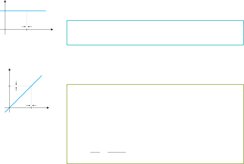
x → a. (See Figure 1.14.) Another simple limit is the following.
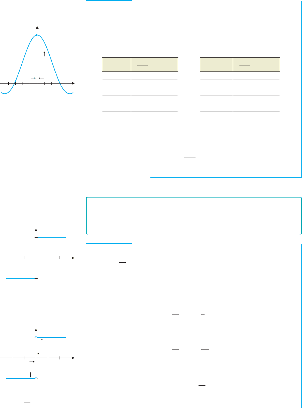
y
x
c
a
xx
y c
FIGURE 1.14
lim
x→a
c = c
For any real number a,
lim
x→a
x = a. (3.2)
Again, this is not a surprise, since as x → a, x will approach a. (See Figure 1.15.) Be
sure that you are comfortable enough with the limit notation to recognize how obvious the
limits in (3.1) and (3.2) are. As simple as they are, we use them repeatedly in finding more
complex limits. We also need the basic rules contained in Theorem 3.1.
y
x
a
f(x)
xx
f(x)
a
y x
FIGURE 1.15
lim
x→a
x = a
THEOREM 3.1
Suppose that lim
x→a
f (x) and lim
x→a
g(x) both exist and let c be any constant. The
following then apply:
(i) lim
x→a
[c · f (x)] = c · lim
x→a
f (x),
(ii) lim
x→a
[ f (x) ± g(x)] = lim
x→a
f (x) ± lim
x→a
g(x),
(iii) lim
x→a
[ f (x) · g(x)] =
lim
x→a
f (x)
lim
x→a
g(x)
and
(iv) lim
x→a
f (x)
g(x)
=
lim
x→a
f (x)
lim
x→a
g(x)
if lim
x→a
g(x) = 0
.
The proof of Theorem 3.1 is found in Appendix A and requires the formal definition of
limit discussed in section 1.6. You should think of theserules as sensible results, given your
intuitive understanding of what a limit is. Read them in plain English. For instance, part (ii)
says that the limit of a sum (or a difference) equals the sum (or difference) of the limits,
provided the limits exist. Think of this as follows. If as x approaches a, f (x) approaches L
and g(x) approaches M, then f (x) + g(x) should approach L + M.
Observe that by applying part (iii) of Theorem 3.1 with g(x) = f (x), we get that,
whenever lim
x→a
f (x) exists,
lim
x→a
[ f (x)]
2
= lim
x→a
[ f (x) · f (x)]
=
lim
x→a
f (x)
lim
x→a
f (x)
=
lim
x→a
f (x)
2
.
Likewise, for any positive integer n, we can apply part (iii) of Theorem 3.1 repeatedly,
to yield
lim
x→a
[ f (x)]
n
=
lim
x→a
f (x)
n
. (3.3)
(See exercises 55 and 56.)
Notice that taking f (x) = x in (3.3) gives us that for any integer n > 0 and any real
number a,
lim
x→a
x
n
= a
n
. (3.4)
That is, to compute the limit of any positive power of x, you simply substitute in the value
of x being approached.

P1: OSO/OVY P2: OSO/OVY QC: OSO/OVY T1: OSO
MHDQ256-Ch01 MHDQ256-Smith-v1.cls December 6, 2010 20:21
LT (Late Transcendental)
CONFIRMING PAGES
1-15 SECTION 1.3
..
Computation of Limits 61
EXAMPLE 3.1 Finding the Limit of a Polynomial
Apply the rules of limits to evaluate lim
x→2
(3x
2
− 5x + 4).
Solution We have
lim
x→2
(3x
2
− 5x + 4) = lim
x→2
(3x
2
) − lim
x→2
(5x) + lim
x→2
4 By Theorem 3.1 (ii).
= 3 lim
x→2
x
2
− 5 lim
x→2
x +4 By Theorem 3.1 (i).
= 3 ·(2)
2
− 5 ·2 +4 = 6. By (3.4).
EXAMPLE 3.2 Finding the Limit of a Rational Function
Apply the rules of limits to evaluate lim
x→3
x
3
− 5x + 4
x
2
− 2
.
Solution We get
lim
x→3
x
3
− 5x + 4
x
2
− 2
=
lim
x→3
(x
3
− 5x + 4)
lim
x→3
(x
2
− 2)
By Theorem 3.1 (iv).
=
lim
x→3
x
3
− 5 lim
x→3
x + lim
x→3
4
lim
x→3
x
2
− lim
x→3
2
By Theorem 3.1 (i) and (ii).
=
3
3
− 5 ·3 +4
3
2
− 2
=
16
7
.
By (3.4).
You may have noticed that in examples 3.1 and 3.2, we simply ended up substituting
the value for x, after taking many intermediate steps. In example 3.3, it’s not quite so
simple.
EXAMPLE 3.3 Finding a Limit by Factoring
Evaluate lim
x→1
x
2
− 1
1 − x
.
Solution Notice right away that
lim
x→1
x
2
− 1
1 − x
=
lim
x→1
(x
2
− 1)
lim
x→1
(1 − x)
,
since the limit in the denominator is zero. (Recall that the limit of a quotient is the
quotient of the limits only when both limits exist and the limit in the denominator is not
zero.) We can resolve this problem by observing that
lim
x→1
x
2
− 1
1 − x
= lim
x→1
(x − 1)(x + 1)
−(x − 1)
Factoring the numerator and
factoring −1 from the denominator.
= lim
x→1
(x + 1)
−1
=−2,
Simplifying and
substituting x = 1.
where the cancellation of the factors of (x − 1) is valid because in the limit as x → 1,
x is close to 1, but x = 1, so that x −1 = 0.
In Theorem 3.2, we show that the limit of a polynomial at a point is simply the value of
the polynomial at that point; that is, to find the limit of a polynomial, we simply substitute
in the value that x is approaching.

P1: OSO/OVY P2: OSO/OVY QC: OSO/OVY T1: OSO
MHDQ256-Ch01 MHDQ256-Smith-v1.cls December 6, 2010 20:21
LT (Late Transcendental)
CONFIRMING PAGES
62 CHAPTER 1
..
Limits and Continuity 1-16
THEOREM 3.2
For any polynomial p(x) and any real number a,
lim
x→a
p(x) = p(a).
PROOF
Suppose that p(x) is a polynomial of degree n ≥ 0,
p(x) = c
n
x
n
+ c
n−1
x
n−1
+···+c
1
x +c
0
.
Then, from Theorem 3.1 and (3.4),
lim
x→a
p(x) = lim
x→a
(c
n
x
n
+ c
n−1
x
n−1
+···+c
1
x +c
0
)
= c
n
lim
x→a
x
n
+ c
n−1
lim
x→a
x
n−1
+···+c
1
lim
x→a
x + lim
x→a
c
0
= c
n
a
n
+ c
n−1
a
n−1
+···+c
1
a + c
0
= p(a).
Evaluating the limit of a polynomial is now easy. Many other limits are evaluated just
as easily.
THEOREM 3.3
Suppose that lim
x→a
f (x) = L and n is any positive integer. Then,
lim
x→a
n
f (x) =
n
lim
x→a
f (x) =
n
L,
where for n even, we must assume that L > 0.
The proof of Theorem 3.3 is given in Appendix A. Notice that this result says that we
may (under the conditions outlined in the hypotheses) bring limits “inside” nth roots. We
can then use our existing rules for computing the limit inside.
EXAMPLE 3.4 Evaluating the Limit of an nth Root of a Polynomial
Evaluate lim
x→2
5
√
3x
2
− 2x.
Solution By Theorems 3.2 and 3.3, we have
lim
x→2
5
3x
2
− 2x =
5
lim
x→2
(3x
2
− 2x) =
5
√
8.
REMARK 3.1
In general, in any case where
the limits of both the numerator
and the denominator are 0, you
should try to algebraically
simplify the expression, to get a
cancellation, as we do in
examples 3.3 and 3.5.
EXAMPLE 3.5 Finding a Limit by Rationalizing
Evaluate lim
x→0
√
x +2 −
√
2
x
.
Solution First, notice that both the numerator and the denominator approach 0 as x
approaches 0. Unlike example 3.3, we can’t factor the numerator. However, we can
rationalize the numerator, as follows:
√
x +2 −
√
2
x
=
(
√
x +2 −
√
2)(
√
x +2 +
√
2)
x(
√
x +2 +
√
2)
=
x +2 −2
x(
√
x +2 +
√
2)
=
x
x(
√
x +2 +
√
2)
=
1
√
x +2 +
√
2
,