Smith R., Minton R. Calculus
Подождите немного. Документ загружается.

P1: OSO/OVY P2: OSO/OVY QC: OSO/OVY T1: OSO
MHDQ256-Ch14 MHDQ256-Smith-v1.cls January 5, 2011 10:17
LT (Late Transcendental)
CONFIRMING PAGES
14-3 SECTION 14.1
..
Double Integrals 903
DEFINITION 1.1
For any function f defined on the interval [a, b], the definite integral of f on [a, b]is
b
a
f (x) dx = lim
P→0
n
i=1
f (c
i
)x
i
,
provided the limit exists and is the same for all choices of the evaluation points
c
i
∈ [x
i−1
, x
i
], for i = 1, 2,...,n. In this case, we say that f is integrable on [a, b].
Here, by saying that the limit in Definition 1.1 equals some value L, we mean that
we can make
n
i=1
f (c
i
)x
i
as close as needed to L, just by making P sufficiently small.
How close must the sum get to L? We must be able to make the sum within any specified
distance ε>0ofL. More precisely, given any ε>0, there must be a δ>0 (depending on
the choice of ε), such that
n
i=1
f (c
i
)x
i
− L
<ε,
for every partition P with P <δ. Notice that this is only a very slight generalization of
our original notion of definite integral. All we have done is to allow the partitions to be
irregular and then defined P to ensure that x
i
→ 0, for every i.
z f(x, y)
z
y
x
R
a
b
d
O
c
FIGURE 14.3
Volume under the surface
z = f (x, y)
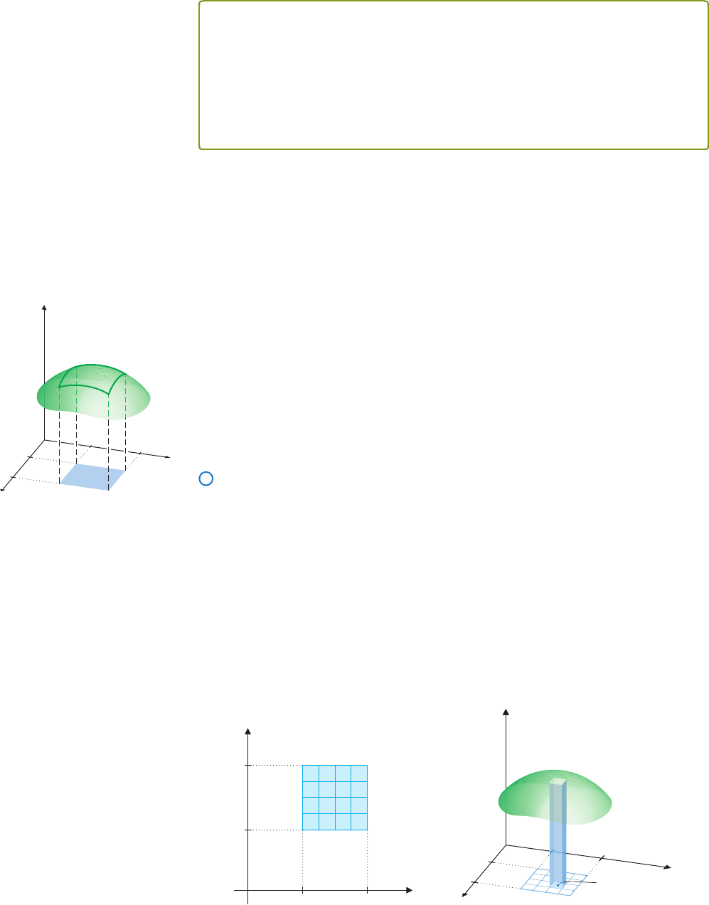
Double Integrals over a Rectangle
For a function f (x, y), where f is continuous and f (x, y) ≥ 0 for all a ≤ x ≤ b and
c ≤ y ≤ d, we wish to find the volume of the solid lying below the surface z = f (x, y)
and above the rectangle R ={(x, y)|a ≤ x ≤ b and c ≤ y ≤ d} in the xy-plane. (See
Figure14.3.)Proceedingessentiallyaswedidtofindtheareaunderacurve,wefirstpartition
the rectangle R by laying down a grid on top of R consisting of n smaller rectangles. (See
Figure 14.4a.) (Note: The rectangles in the grid need not be all of the same size.) Call the
smaller rectangles R
1
, R
2
,...,R
n
. (The order in which you number them is irrelevent.)
For each rectangle R
i
(i = 1, 2,...,n) in the partition, we approximate the volume V
i
lying beneath the surface z = f (x, y) and above the rectangle R
i
by constructing a rect-
angular box whose height is f (u
i
,v
i
), for some point (u
i
,v
i
) ∈ R
i
. (See Figure 14.4b.)
y
x
ba
c
d
R
i
z f(x, y)
(u
i
, v
i
)
z
O
y
x
a
b
d
c
FIGURE 14.4a FIGURE 14.4b
Partition of R Approximating the volume above
R
i
by a rectangular box
P1: OSO/OVY P2: OSO/OVY QC: OSO/OVY T1: OSO
MHDQ256-Ch14 MHDQ256-Smith-v1.cls January 5, 2011 10:17
LT (Late Transcendental)
CONFIRMING PAGES
904 CHAPTER 14
..
Multiple Integrals 14-4
z f(x, y)
z
O
y
x
a
b
d
c
z f (x, y)
z
O
y
x
a
b
d
c
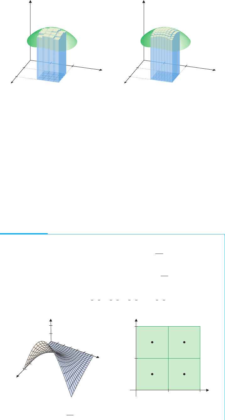
FIGURE 14.4c FIGURE 14.4d
Approximate volume Approximate volume
Notice that the volume V
i
beneath the surface z = f (x, y) and above R
i
is approximated
by the volume of the box:
V
i
≈ Height × Area of base = f (u
i
,v
i
) A
i
,
where A
i
denotes the area of the rectangle R
i
.
The total volume is then approximately
V ≈
n
i=1
f (u
i
,v
i
) A
i
. (1.2)
As in our development of the definite integral in Chapter 4, we call the sum in (1.2) a
Riemann sum. We illustrate the approximation of the volumeunder a surfaceby aRiemann
sum in Figures 14.4c and 14.4d. Notice that the larger number of rectangles used in Figure
14.4d appears to give a better approximation of the volume.
EXAMPLE 1.1 Approximating the Volume Lying Beneath a Surface
Approximate the volume lying beneath the surface z = x
2
sin
π y
6
and above the
rectangle R ={(x, y)|0 ≤ x ≤ 6, 0 ≤ y ≤ 6}.
Solution First, note that f is continuous and f (x, y) = x
2
sin
π y
6
≥ 0onR. (See
Figure 14.5a.) Next, a simple partition of R is a partition into four squares of equal size,
as indicated in Figure 14.5b. We choose the evaluation points (u
i
,v
i
) to be the centers
of each of the four squares, that is,
3
2
,
3
2
,
9
2
,
3
2
,
3
2
,
9
2
and
9
2
,
9
2
.
z
y
x
20
2
6
4
6
y
x
R
3
R
4
R
1
R
2
3
6
3 6
O
FIGURE 14.5a FIGURE 14.5b
z = x
2
sin
π y
6
Partition of R into four equal squares
P1: OSO/OVY P2: OSO/OVY QC: OSO/OVY T1: OSO
MHDQ256-Ch14 MHDQ256-Smith-v1.cls January 5, 2011 10:17
LT (Late Transcendental)
CONFIRMING PAGES
14-5 SECTION 14.1
..
Double Integrals 905
Since the four squares are the same size, we have A
i
= 9, for each i.For
f (x, y) = x
2
sin
π y
6
, we have from (1.2) that
V ≈
4
i=1
f (u
i
,v
i
) A
i
= f
3
2
,
3
2
(9) + f
9
2
,
3
2
(9) + f
3
2
,
9
2
(9) + f
9
2
,
9
2
(9)
= 9
3
2
2
sin
π
4
+
9
2
2
sin
π
4
+
3
2
2
sin
3π
4
+
9
2
2
sin
3π
4
=
405
2
√
2 ≈ 286.38.
R
1
R
2
R
3
R
4
O
R
5
R
6
R
7
R
8
R
9
6
y
x
4
2
6
2 4
FIGURE 14.5c
Partition of R into nine equal squares
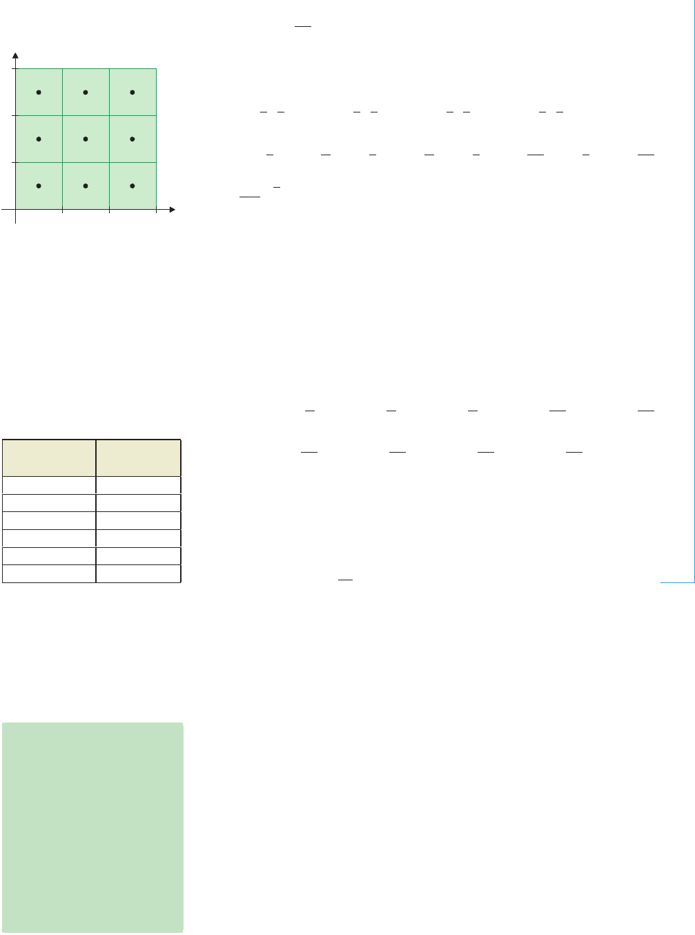
We can improve on this approximation by increasing the number of rectangles in the
partition. For instance, partitioning R into nine squares of equal size (as in Figure 14.5c)
and again using the center of each square as the evaluation point, we have A
i
= 4 for
each i and
V ≈
9
i=1
f (u
i
,v
i
) A
i
= 4[f (1, 1) + f (3, 1) + f (5, 1) + f (1, 3) + f (3, 3) + f (5, 3)
+ f (1, 5) + f (3, 5) + f (5, 5)]
= 4
1
2
sin
π
6
+ 3
2
sin
π
6
+ 5
2
sin
π
6
+ 1
2
sin
3π
6
+ 3
2
sin
3π
6
+5
2
sin
3π
6
+ 1
2
sin
5π
6
+ 3
2
sin
5π
6
+ 5
2
sin
5π
6
= 280.
Continuing in this fashion to divide R into more and more squares of equal size and
using the center of each square as the evaluation point, we construct increasingly better
and better approximations of the volume. (See the table in the margin.) From the table,
it appears that a reasonable approximation to the volume is slightly less than 275.07. In
fact, the exact volume is
864
π
≈ 275.02. (We’ll show you how to find this shortly.)
No. of Squares Approximate
in Partition Volume
4 286.38
9 280.00
36 276.25
144 275.33
400 275.13
900 275.07
NOTES
The choice of the center of each
square as the evaluation point, as
used in example 1.1, corresponds
to the Midpoint rule for
approximating the value of a
definite integral for a function of
a single variable (discussed in
section 4.7). This choice of
evaluation points generally
produces a reasonably good
approximation.
Turning (1.2) intoan exact formula for volume takes more than simply letting n →∞,
since we need to have all of the rectangles in the partition shrink to zero area. A convenient
way of doing this is to define the norm of the partition P to be the largest diagonal of
any rectangle in the partition. Note that if P→0, then all of the rectangles must shrink
to zero area. We can now make the volume approximation (1.2) exact:
V = lim
P→0
n
i=1
f (u
i
,v
i
) A
i
,
assuming the limit exists and is the same for every choice of the evaluation points. Here,
by saying that this limit equals V, we mean that we can make
n
i=1
f (u
i
,v
i
) A
i
as close as
needed to V, just by making Psufficiently small. More precisely, this says that given any
ε>0, there is a δ>0 (depending on the choice of ε), such that
n
i=1
f (u
i
,v
i
) A
i
− V
<ε,
forevery partition P with P <δ.More generally, wehave the followingdefinition, which
applies even when the function takes on negative values.
P1: OSO/OVY P2: OSO/OVY QC: OSO/OVY T1: OSO
MHDQ256-Ch14 MHDQ256-Smith-v1.cls January 5, 2011 10:17
LT (Late Transcendental)
CONFIRMING PAGES
906 CHAPTER 14
..
Multiple Integrals 14-6
DEFINITION 1.2
For any function f defined on the rectangle
R ={(x, y)|a ≤ x ≤ b and c ≤ y ≤ d}, we define the double integral of f over R by
R
f (x, y) dA = lim
P→0
n
i=1
f (u
i
,v
i
) A
i
,
providedthelimit existsand isthesamefor everychoiceofthe evaluationpoints (u
i
,v
i
)
in R
i
, for i = 1, 2,...,n. When this happens, we say that f is integrable over R.
REMARK 1.1
It can be shown that if f is
continuous on R, then it is also
integrable over R. The proof can
be found in more advanced
texts.
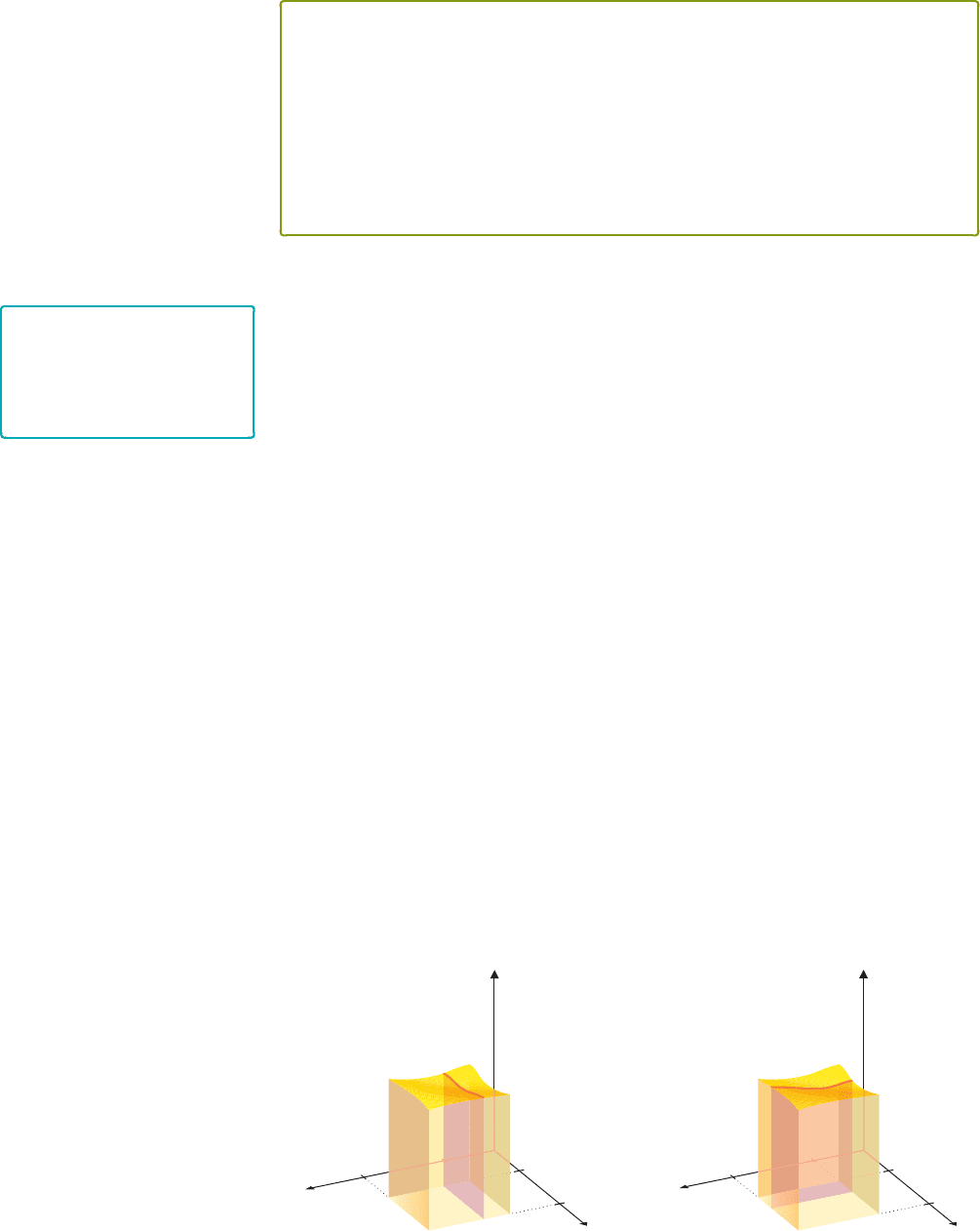
Note that just as when we first defined the definite integral of a function of one variable,
we don’t yet know how to compute this double integral. We first consider the special case
where f (x, y) ≥ 0 on the rectangle R ={(x, y)|a ≤ x ≤ b and c ≤ y ≤ d}. Notice that
here,
R
f (x, y) dA represents the volume lying beneath the surface z = f (x, y) and above
the region R. Recall that we already know how to compute this volume, from our work
in section 5.2. We can do this by slicing the solid with planes parallel to the yz-plane, as
indicated in Figure 14.6a. If we denote the area of the cross section of the solid for a given
value of x by A(x), then we have from equation (2.1) in section 5.2 that the volume is
given by
V =
b
a
A(x)dx.
Now, note that for each fixed value of x, the area of the cross section is simply the area under
the curve z = f (x, y) for c ≤ y ≤ d, which is given by the integral
A(x) =
d
c
f (x, y) dy.
This integration is called a partial integration with respect to y, since x is held fixed and
f (x, y) is integrated with respect to y. This leaves us with
V =
b
a
A(x)dx =
b
a
d
c
f (x, y) dy
dx. (1.3)
Likewise, if we instead slice the solid with planes parallel to the xz-plane, as indicated in
Figure 14.6b, we get that the volume is given by
V =
d
c
A(y)dy =
d
c
b
a
f (x, y) dx
dy. (1.4)
x
y
z
z f (x, y)
O
R
A(x)
a
b
d
c
x
y
z
z f (x, y)
O
R
a
b
d
c
A(y)
FIGURE 14.6a FIGURE 14.6b
Slicing the solid parallel to the Slicing the solid parallel to the
yz-plane xz-plane

P1: OSO/OVY P2: OSO/OVY QC: OSO/OVY T1: OSO
MHDQ256-Ch14 MHDQ256-Smith-v1.cls January 5, 2011 10:17
LT (Late Transcendental)
CONFIRMING PAGES
14-7 SECTION 14.1
..
Double Integrals 907
The integrals in (1.3) and (1.4) are called iterated integrals. Note that each of these
indicates a partial integration with respect to the inner variable (i.e., you first integrate with
respect to the inner variable, treating the outer variable as a constant), to be followed by an
integration with respect to the outer variable.
For simplicity, we ordinarily write the iterated integrals without the brackets:
b
a
d
c
f (x, y) dy
dx =
b
a
d
c
f (x, y) dy dx
and
d
c
b
a
f (x, y) dx
dy =
d
c
b
a
f (x, y) dx dy.
Asindicated,theseintegralsare evaluatedinsideout,usingthemethodsofintegrationwe’ve
already established for functions of a single variable. This now establishes the following
result for the special case where f (x, y) ≥ 0. The proof of the result for the general case is
rather lengthy and we omit it.
HISTORICAL
NOTES
Guido Fubini (1879–1943)
Italian mathematician who made
wide-ranging contributions to
mathematics, physics and
engineering. Fubini’s early work
was in differential geometry, but
he quickly diversified his research
to include analysis, the calculus
of variations, group theory,
non-Euclidean geometry and
mathematical physics.
Mathematics was the family
business, as his father was a
mathematics teacher and his sons
became engineers. Fubini moved
to the United States in 1939 to
escape the persecution of Jews in
Italy. He was working on an
engineering textbook inspired by
his sons’ work when he died.
THEOREM 1.1 (Fubini’s Theorem)
Suppose that f is integrable over the rectangle R ={(x, y)|a ≤ x ≤ b and c ≤ y ≤ d}.
Then we can write the double integral of f over R as either of the iterated integrals:
R
f (x, y) dA =
b
a
d
c
f (x, y) dydx =
d
c
b
a
f (x, y) dx dy. (1.5)
Fubini’s Theorem simply tells you that you can always rewrite a double integral over
a rectangle as either one of a pair of iterated integrals. We illustrate this in example 1.2.
EXAMPLE 1.2 Double Integral over a Rectangle
If R ={(x, y)|0 ≤ x ≤ 2 and 1 ≤ y ≤ 4}, evaluate
R
(6x
2
+ 4xy
3
)dA.
Solution From (1.5), we have
R
(6x
2
+ 4xy
3
)dA =
4
1
2
0
(6x
2
+ 4xy
3
)dx dy
=
4
1
2
0
(6x
2
+ 4xy
3
)dx
dy
=
4
1
6
x
3
3
+ 4
x
2
2
y
3
x=2
x=0
dy
=
4
1
(16 + 8y
3
)dy
=
16y + 8
y
4
4
4
1
= [16(4) +2(4)
4
] − [16(1) + 2(1)
4
] = 558.
Note that we evaluated the first integral above by integrating with respect to x, while
treating y as a constant. We leave it as an exercise to show that you get the same value
by integrating first with respect to y, that is, that
R
(6x
2
+ 4xy
3
)dA =
2
0
4
1
(6x
2
+ 4xy
3
)dy dx = 558,
also.
P1: OSO/OVY P2: OSO/OVY QC: OSO/OVY T1: OSO
MHDQ256-Ch14 MHDQ256-Smith-v1.cls January 5, 2011 10:17
LT (Late Transcendental)
CONFIRMING PAGES
908 CHAPTER 14
..
Multiple Integrals 14-8
Double Integrals over General Regions
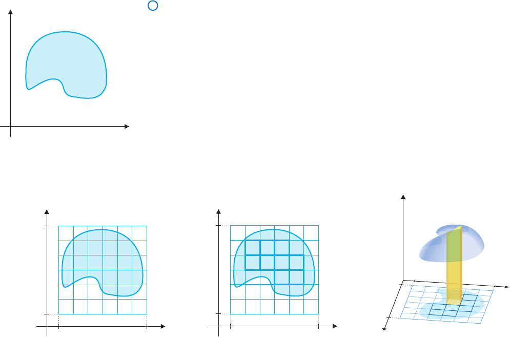
We now wish to extend the notion of double integral to a bounded, nonrectangular region
like the one shown in Figure 14.7a. (Recall that a region is bounded if it fits inside a circle
of some finite radius.) We begin, as we did for the case of rectangular regions, by looking
for the volume lying beneath the surface z = f (x, y) and lying above the region R, where
f (x, y) ≥ 0 and f is continuous on R.
First, notice that the grid we used initially to partition a rectangular region must be
modified, since such a rectangular grid won’t “fit” a nonrectangular region, as shown
in Figure 14.7b. We resolve this problem by considering only those rectangular sub-
regions that lie completely inside the region R. (See Figure 14.7c, where we have
labeled these rectangles.) We call the collection of these rectangles an inner parti-
tion of R. For instance, in the inner partition indicated in Figure 14.7c, there are nine
subregions.
y
x
R
FIGURE 14.7a
Nonrectangular region
y
x
ba
c
d
R
y
x
ba
c
d
R
1
R
2
R
3
R
4
R
5
R
6
R
7
R
8
R
9
x
y
z
O
FIGURE 14.7b FIGURE 14.7c FIGURE 14.7d
Grid for a general region Inner partition Sample volume box
Fromthispointon,weproceedessentiallyaswedidforthecaseofarectangularregion.
Thatis,oneachrectangularsubregion R
i
(i = 1, 2,...,n)inaninnerpartition,weconstruct
a rectangular box of height f (u
i
,v
i
), for some point (u
i
,v
i
) ∈ R
i
. (See Figure 14.7d for a
sample box.) The volume V
i
beneath the surface and above R
i
is then approximately
V
i
≈ Height × Area of base = f (u
i
,v
i
) A
i
,
where we again denote the area of R
i
by A
i
. The total volume V lying beneath the surface
and above the region R is then approximately
V ≈
n
i=1
f (u
i
,v
i
) A
i
. (1.6)
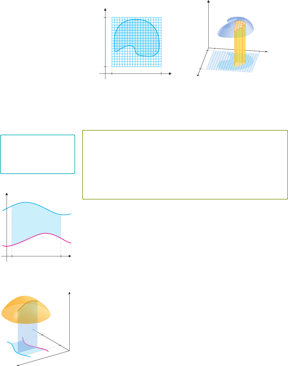
We define the norm of the inner partition P to be the length of the largest diago-
nal of any of the rectangles R
1
, R
2
,...,R
n
. Notice that as we make P smaller and
smaller, the inner partition fills in R nicely (as in Figure 14.8a) and the approximate volume
given by (1.6) should get closer and closer to the actual volume. (See Figure 14.8b.) We
then have
V = lim
||P||→0
n
i=1
f (u
i
,v
i
) A
i
,
assuming the limit exists and is the same for every choice of the evaluation points.
P1: OSO/OVY P2: OSO/OVY QC: OSO/OVY T1: OSO
MHDQ256-Ch14 MHDQ256-Smith-v1.cls January 5, 2011 10:17
LT (Late Transcendental)
CONFIRMING PAGES
14-9 SECTION 14.1
..
Double Integrals 909
y
x
ba
c
d
x
y
z
O
FIGURE 14.8a FIGURE 14.8b
Refined grid Approximate volume
More generally, we have Definition 1.3.
DEFINITION 1.3
For any function f defined on a bounded region R ⊂ R
2
, we define the double
integral of f over R by
R
f (x, y) dA = lim
P→0
n
i=1
f (u
i
,v
i
) A
i
, (1.7)
provided the limit exists and is the same for every choice of the evaluation points
(u
i
,v
i
)inR
i
, for i = 1, 2,...,n. In this case, we say that f is integrable over R.
REMARK 1.2
Once again, it can be shown that
if f is continuous on R, then it is
integrable over R, although the
proof is beyond the level of this
course.
y
R
x
a b
y g
2
(x)
y g
1
(x)
FIGURE 14.9a
The region R
a
b
R
z
y
x
z f (x, y)
O
A(x)
FIGURE 14.9b
Volume by slicing
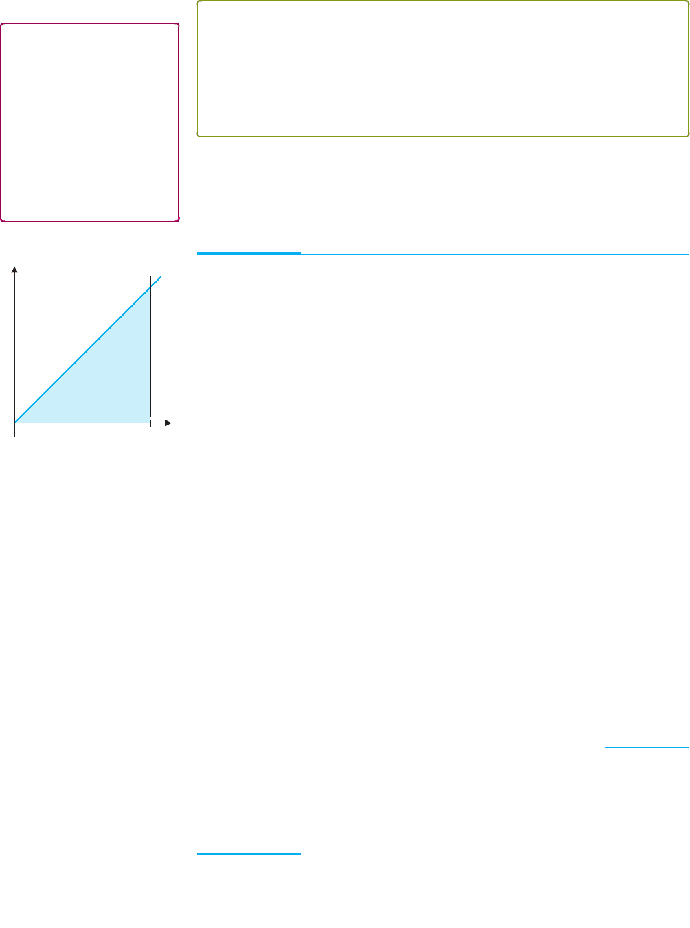
Calculating a double integral over a nonrectangular region is a bit more complicated
than it was for the case of a rectangular region and depends on the exact form of R. We first
consider the case where the region R lies between the vertical lines x = a and x = b, with
a < b, has a top defined by the curve y = g
2
(x) and a bottom defined by y = g
1
(x), where
g
1
(x) ≤ g
2
(x) for all x in (a, b). That is, R has the form
R ={(x, y)|a ≤ x ≤ b and g
1
(x) ≤ y ≤ g
2
(x)}.
See Figure 14.9a for a typical region of this form lying in the first quadrant of the xy-plane.
Think about this for the special case where f (x, y) ≥ 0onR. Here, the double integral of
f over R gives the volume lying beneath the surface z = f (x, y) and above the region R in
the xy-plane. We can find this volume by the method of slicing, just as we did for the case
of a double integral over a rectangular region.
From Figure 14.9b, observe that for each fixed x ∈ [a, b], the area of the slice lying
above the line segment indicated and below the surface z = f (x, y)isgivenby
A(x) =
g
2
(x)
g
1
(x)
f (x, y) dy.
The volume of the solid is then given by equation (2.1) in section 5.2 to be
V =
b
a
A(x)dx =
b
a
g
2
(x)
g
1
(x)
f (x, y) dy dx.
Recognizingthe volumeas V =
R
f (x, y) dA proves thefollowingtheorem,forthespecial
case where f (x, y) ≥ 0onR.
P1: OSO/OVY P2: OSO/OVY QC: OSO/OVY T1: OSO
MHDQ256-Ch14 MHDQ256-Smith-v1.cls January 7, 2011 7:53
LT (Late Transcendental)
CONFIRMING PAGES
910 CHAPTER 14
..
Multiple Integrals 14-10
THEOREM 1.2
Suppose that f is continuous on the region R defined by
R ={(x, y)|a ≤ x ≤ b and g
1
(x) ≤ y ≤ g
2
(x)}, for continuous functions g
1
and g
2
,
where g
1
(x) ≤ g
2
(x), for all x in [a, b]. Then,
R
f (x, y) dA =
b
a
g
2
(x)
g
1
(x)
f (x, y) dy dx.
CAUTION
Be sure to draw a reasonably
good sketch of the region R
before you try to write down the
iterated integrals. Without doing
this, you may be lucky enough
(or clever enough) to get the
first few exercises to work out,
but you will ultimately be
doomed to failure. It is essential
that you have a clear picture of
the region in order to set up the
integrals correctly.
AlthoughthegeneralproofofTheorem1.2is beyondthelevelofthistext,the derivation
given above for the special case where f (x, y) ≥ 0 should help to make some sense of this.
We illustrate the process of writing a double integral as an iterated integral in
example 1.3.
EXAMPLE 1.3 Evaluating a Double Integral
Let R be the region bounded by the graphs of y = x, y = 0 and x = 4. Evaluate
R
(4e
x
2
− 5 sin y)dA.
y
4
y ⫽ x
y ⫽ 0
R
x
FIGURE 14.10
The region R
Solution First, we draw a graph of the region R in Figure 14.10. To help with
determining the limits of integration, we have drawn a line segment illustrating that for
each fixed value of x on the interval [0, 4], the y-values range from 0 up to x. From
Theorem 1.2, we have
R
(4e
x
2
− 5 sin y)dA =
4
0
x
0
(4e
x
2
− 5 sin y)dy dx (1.8)
=
4
0
(4ye
x
2
+ 5 cos y)
y=x
y=0
dx
=
4
0
(4xe
x
2
+ 5 cos x −5) dx
= (2e
x
2
+ 5 sin x −5x)
4
0
= 2e
16
+ 5 sin4 −22 ≈ 1.78 × 10
7
.
Be very careful here; there are plenty of traps to fall into. The most common error
is to simply look for the minimum and maximum values of x and y and mistakenly write
R
f (x, y) dA =
4
0
4
0
f (x, y) dy dx. This is incorrect!
Notice that instead of integrating over the region R shown in Figure 14.10, as in (1.8),
this corresponds to integration over the rectangle 0 ≤ x ≤ 4, 0 ≤ y ≤ 4.
As with any other integral, iterated integrals often cannot be evaluated symbolically
(even with a very good computer algebra system). In such cases, we must rely on approxi-
mate methods. This is easily accomplished if you evaluate the inner integral symbolically
and then use a numerical method (e.g., Simpson’s Rule) to approximate the outer integral.
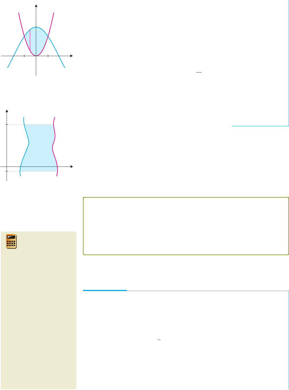
EXAMPLE 1.4 Approximate Limits of Integration
Evaluate
R
(x
2
+ 6y)dA, where R is the region bounded by the graphs of y = cos x
and y = x
2
.
P1: OSO/OVY P2: OSO/OVY QC: OSO/OVY T1: OSO
MHDQ256-Ch14 MHDQ256-Smith-v1.cls January 5, 2011 10:17
LT (Late Transcendental)
CONFIRMING PAGES
14-11 SECTION 14.1
..
Double Integrals 911
Solution Notice that the inner limits of integration are easy to see from Figure 14.11;
for each fixed x, y ranges from x
2
up to cos x. To find the outer limits, we must find the
intersections of the two curves by solving the equation cosx = x
2
. We can’t solve this
exactly, but using a numerical procedure (e.g., Newton’s method or one built into your
calculator or computer algebra system), we get approximate intersections of
x ≈±0.82413. From Theorem 1.2, we now have
R
(x
2
+ 6y)dA ≈
0.82413
−0.82413
cos x
x
2
(x
2
+ 6y)dy dx
=
0.82413
−0.82413
x
2
y + 6
y
2
2
y=cos x
y=x
2
dx
=
0.82413
−0.82413
[(x
2
cos x + 3cos
2
x) −(x
4
+ 3x
4
)]dx
≈ 3.659765588,
where we have evaluated the last integral approximately, even though it could be done
exactly, using integration by parts and a trigonometric identity.
y
x
0.824 . . .0.824 . . .
y cos x
y x
2
R
FIGURE 14.11
The region R
y
x
d
c
x h
1
(y)
x h
2
(y)
R
FIGURE 14.12
Typical region
Not all double integrals can be computed using the technique of examples 1.3 and 1.4.
Often, it is necessary (or at least convenient) to think of the geometry of the region R in a
different way.
Suppose that the region R has the form
R ={(x, y)|c ≤ y ≤ d and h
1
(y) ≤ x ≤ h
2
(y)},
as indicated in Figure 14.12. Then, much as in Theorem 1.2, we can write double integrals
as iterated integrals, as in Theorem 1.3.
THEOREM 1.3
Suppose that f is continuous on the region R defined by
R ={(x, y)|c ≤ y ≤ d and h
1
(y) ≤ x ≤ h
2
(y)}, for continuous functions h
1
and h
2
,
where h
1
(y) ≤ h
2
(y), for all y in [c, d]. Then,
R
f (x, y) dA =
d
c
h
2
(y)
h
1
(y)
f (x, y) dx dy.
TODAY IN
MATHEMATICS
Mary Ellen Rudin (1924– )
An American mathematician who
published more than 70 research
papers while supervising Ph.D.
students, raising four children and
earning the love and respect of
students and colleagues. As a
child, she and her friends played
games that were “very elaborate
and purely in the imagination.
I think actually that that is
something that contributes to
making a mathematician—having
time to think and being in the
habit of imagining all sorts of
complicated things.” She says,
“I’m very geometric in my
thinking. I’m not really interested
in numbers.” She describes her
teaching style as, “I bubble and I
get students enthusiastic.”
The general proof of this theorem is beyond the level of this course, although the
reasonablenessofthisresultshouldbeapparentfromTheorem1.2andtheanalysispreceding
that theorem, for the special case where f (x, y) ≥ 0onR.
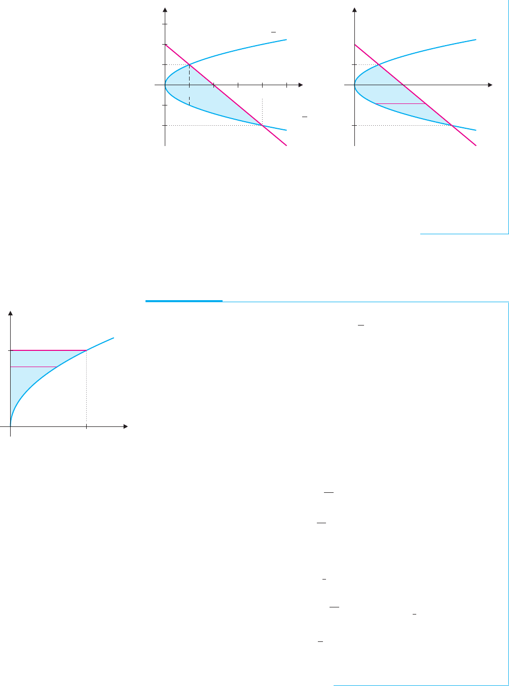
EXAMPLE 1.5 Integrating First with Respect to x
Write
R
f (x, y) dA as an iterated integral, where R is the region bounded by the graphs
of x = y
2
and x = 2 − y.
Solution From the graph of the region in Figure 14.13a (on the following page),
notice that integrating first with respect to y is not a very good choice, since the upper
boundary of the region is y =
√
x for 0 ≤ x ≤ 1 and y = 2 − x for 1 ≤ x ≤ 4. A more
reasonable choice is to use Theorem 1.3 and integrate first with respect to x. In Figure
14.13b (on the following page), we have included a horizontal line segment indicating
the inner limits of integration: for each fixed y, x runs from x = y
2
over to x = 2 − y.
The value of y then runs between the values at the intersections of the two curves. To
find these, we solve y
2
= 2 − y or
0 = y
2
+ y −2 = (y +2) (y − 1),
P1: OSO/OVY P2: OSO/OVY QC: OSO/OVY T1: OSO
MHDQ256-Ch14 MHDQ256-Smith-v1.cls January 5, 2011 10:17
LT (Late Transcendental)
CONFIRMING PAGES
912 CHAPTER 14
..
Multiple Integrals 14-12
1 2 3 4 5
1
2
1
2
3
y 2 x
y
R
x
y x
y x
2
1
y
x
x 2 y
x y
2
R
FIGURE 14.13a FIGURE 14.13b
The region R The region R
so that the intersections are at y =−2 and y = 1. From Theorem 1.3, we now have
R
f (x, y) dA =
1
−2
2−y
y
2
f (x, y) dx dy.
y
x
9
3
x y
2
R
FIGURE 14.14
The region R
You will often have to choose which variable to integrate with respect to first. Some-
times, you make your choice on the basis of the region. Often, a double integral can be set
up either way but is much easier to calculate one way than the other. This is the case in
example 1.6.
EXAMPLE 1.6 Evaluating a Double Integral
Let R be the region bounded by the graphs of y =
√
x, x = 0 and y = 3. Evaluate
R
(2xy
2
+ 2y cosx)dA.
Solution We show a graph of the region in Figure 14.14. From Theorem 1.3, we have
R
(2xy
2
+ 2y cosx)dA =
3
0
y
2
0
(2xy
2
+ 2y cosx)dx dy
=
3
0
(x
2
y
2
+ 2y sinx)
x=y
2
x=0
dy
=
3
0
(y
6
+ 2y sin y
2
)dy
=
y
7
7
− cos y
2
3
0
=
3
7
7
− cos 9 +cos0 ≈ 314.3.
Alternatively, integrating with respect to y first, we get
R
(2xy
2
+ 2y cosx)dA =
9
0
3
√
x
(2xy
2
+ 2y cosx)dydx
=
9
0
2x
y
3
3
+ y
2
cos x
y=3
y=
√
x
dx
=
9
0
2
3
x(27 − x
3/2
) + (3
2
− x) cos x
dx,
which leaves you with an integration by parts to carry out. We leave the details as an
exercise. Which way do you think is easier?