Thomas M. Cover, Joy A. Thomas. Elements of information theory
Подождите немного. Документ загружается.


11.5 EXAMPLES OF SANOV’S THEOREM 365
From (11.110), it follows that P
∗
has the form
P
∗
(x) =
2
λx
6
i=1
2
λi
, (11.113)
with λ chosen so that
iP
∗
(i) = 4. Solving numerically, we obtain
λ = 0.2519, P
∗
= (0.1031, 0.1227, 0.1461, 0.1740, 0.2072, 0.2468),and
therefore D(P
∗
||Q) = 0.0624 bit. Thus, the probability that the average
of 10000 throws is greater than or equal to 4 is ≈ 2
−624
.
Example 11.5.2 (C oins) Suppose that we have a fair coin and want
to estimate the probability of observing more than 700 heads in a series
of 1000 tosses. The problem is like Example 11.5.1. The probability is
P(
X
n
≥ 0.7)
.
= 2
−nD(P
∗
||Q)
, (11.114)
where P
∗
is the (0.7, 0.3) distribution and Q is the (0.5, 0.5) distribution.
In this case, D(P
∗
||Q) = 1 −H(P
∗
) = 1 − H(0.7) = 0.119. Thus, the
probability of 700 or more heads in 1000 trials is approximately 2
−119
.
Example 11.5.3 (Mutual dependence)LetQ(x, y) be a given joint
distribution and let Q
0
(x, y) = Q(x)Q(y) be the associated product dis-
tribution formed from the marginals of Q. We wish to know the likelihood
that a sample drawn according to Q
0
will “appear” to be jointly dis-
tributed according to Q. Accordingly, let (X
i
,Y
i
) be i.i.d. ∼ Q
0
(x, y) =
Q(x)Q(y). We define joint typicality as we did in Section 7.6; that is,
(x
n
,y
n
) is jointly typical with respect to a joint distribution Q(x, y) iff
the sample entropies are close to their true values:
−
1
n
log Q(x
n
) − H(X)
≤ , (11.115)
−
1
n
log Q(y
n
) − H(Y)
≤ , (11.116)
and
−
1
n
log Q(x
n
,y
n
) − H(X,Y)
≤ . (11.117)
We wish to calculate the probability (under the product distribution) of
seeing a pair (x
n
,y
n
) that looks jointly typical of Q [i.e., (x
n
,y
n
)
366 INFORMATION THEORY AND STATISTICS
satisfies (11.115)–(11.117)]. Thus, (x
n
,y
n
) are jointly typical with respect
to Q(x, y) if P
x
n
,y
n
∈ E ∩ P
n
(X, Y ),where
E ={P(x, y) :
−
x,y
P(x, y) log Q(x) − H(X)
≤ ,
−
x,y
P(x, y) log Q(y) − H(Y)
≤ ,
−
x,y
P(x, y) log Q(x, y) − H(X,Y)
≤ }. (11.118)
Using Sanov’s theorem, the probability is
Q
n
0
(E)
.
= 2
−nD(P
∗
||Q
0
)
, (11.119)
where P
∗
is the distribution satisfying the constraints that is closest to
Q
0
in relative entropy. In this case, as → 0, it can be verified (Prob-
lem 11.10) that P
∗
is the joint distribution Q,andQ
0
is the product
distribution, so that the probability is 2
−nD(Q(x,y)||Q(x)Q(y))
= 2
−nI (X;Y)
,
which is the same as the result derived in Chapter 7 for the joint AEP.
In the next section we consider the empirical distribution of the sequence
of outcomes given that the type is in a particular set of distributions E.We
will show that not only is the probability of the set E essentially determined
by D(P
∗
||Q), the distance of the closest element of E to Q, but also that
the conditional type is essentially P
∗
, so that given that we are in set E,the
type is very likely to be close to P
∗
.
11.6 CONDITIONAL LIMIT THEOREM
It has been shown that the probability of a set of types under a distribution
Q is determined essentially by the probability of the closest element of
the set to Q; the probability is 2
−nD
∗
to first order in the exponent, where
D
∗
= min
P ∈E
D(P ||Q). (11.120)
This follows because the probability of the set of types is the sum of the
probabilities of each type, which is bounded by the largest term times the
11.6 CONDITIONAL LIMIT THEOREM 367
E
Q
P
P
*
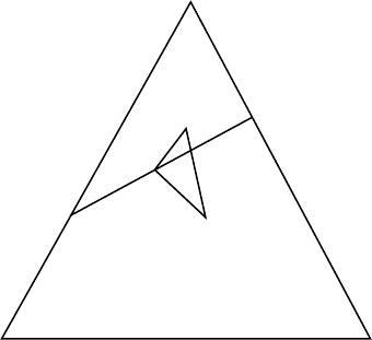
FIGURE 11.5. Pythagorean theorem for relative entropy.
number of terms. Since the number of terms is polynomial in the length
of the sequences, the sum is equal to the largest term to first order in the
exponent.
We now strengthen the argument to show that not only is the proba-
bility of the set E essentially the same as the probability of the closest
type P
∗
but also that the total probability of other types that are far
away from P
∗
is negligible. This implies that with very high probabil-
ity, the type observed is close to P
∗
. We call this a conditional limit
theorem.
Before we prove this result, we prove a “Pythagorean” theorem, which
gives some insight into the geometry of D(P ||Q).SinceD(P ||Q) is not
a metric, many of the intuitive properties of distance are not valid for
D(P ||Q). The next theorem shows a sense in which D(P ||Q) behaves
like the square of the Euclidean metric (Figure 11.5).
Theorem 11.6.1 For a closed convex set E ⊂
P and distribution Q/∈
E,letP
∗
∈ E be the distribution that achieves the minimum distance to
Q; that is,
D(P
∗
||Q) = min
P ∈E
D(P ||Q). (11.121)
Then
D(P ||Q) ≥ D(P ||P
∗
) + D(P
∗
||Q) (11.122)
for all P ∈ E.

368 INFORMATION THEORY AND STATISTICS
Note.
The main use of this theorem is as follows: Suppose that we have
a sequence P
n
∈ E that yields D(P
n
||Q) → D(P
∗
||Q). Then from the
Pythagorean theorem, D(P
n
||P
∗
) → 0 as well.
Proof: Consider any P ∈ E.Let
P
λ
= λP + (1 − λ)P
∗
. (11.123)
Then P
λ
→ P
∗
as λ → 0. Also, since E is convex, P
λ
∈ E for 0 ≤ λ ≤ 1.
Since D(P
∗
||Q) is the minimum of D(P
λ
||Q) along the path P
∗
→ P ,
the derivative of D(P
λ
||Q) as a function of λ is nonnegative at λ = 0.
Now
D
λ
= D(P
λ
||Q) =
P
λ
(x) log
P
λ
(x)
Q(x)
(11.124)
and
dD
λ
dλ
=
(P (x) − P
∗
(x)) log
P
λ
(x)
Q(x)
+ (P (x) − P
∗
(x))
. (11.125)
Setting λ = 0, so that P
λ
= P
∗
and using the fact that
P(x) =
P
∗
(x) = 1, we have
0 ≤
dD
λ
dλ
λ=0
(11.126)
=
(P (x) − P
∗
(x)) log
P
∗
(x)
Q(x)
(11.127)
=
P(x)log
P
∗
(x)
Q(x)
−
P
∗
(x) log
P
∗
(x)
Q(x)
(11.128)
=
P(x)log
P(x)
Q(x)
P
∗
(x)
P(x)
−
P
∗
(x) log
P
∗
(x)
Q(x)
(11.129)
= D(P ||Q) − D(P||P
∗
) − D(P
∗
||Q), (11.130)
which proves the theorem.
Note that the relative entropy D(P ||Q) behaves like the square of the
Euclidean distance. Suppose that we have a convex set E in
R
n
.LetA
be a point outside the set, B the point in the set closest to A,andC any
11.6 CONDITIONAL LIMIT THEOREM 369
A
B
C
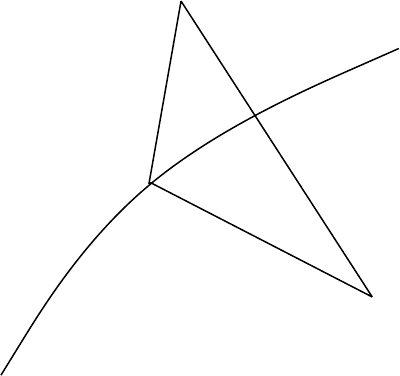
FIGURE 11.6. Triangle inequality for distance squared.
other point in the set. Then the angle between the lines BA and BC must
be obtuse, which implies that l
2
AC
≥ l
2
AB
+ l
2
BC
, which is of the same form
as Theorem 11.6.1. This is illustrated in Figure 11.6.
We now prove a useful lemma which shows that convergence in relative
entropy implies convergence in the
L
1
norm.
Definition The
L
1
distance between any two distributions is defined as
||P
1
− P
2
||
1
=
a∈X
|P
1
(a) − P
2
(a)|. (11.131)
Let A be the set on which P
1
(x) > P
2
(x).Then
||P
1
− P
2
||
1
=
x∈X
|P
1
(x) − P
2
(x)| (11.132)
=
x∈A
(P
1
(x) − P
2
(x)) +
x∈A
c
(P
2
(x) − P
1
(x)) (11.133)
= P
1
(A) − P
2
(A) + P
2
(A
c
) − P
1
(A
c
) (11.134)
= P
1
(A) − P
2
(A) + 1 −P
2
(A) − 1 +P
1
(A) (11.135)
= 2(P
1
(A) − P
2
(A)). (11.136)

370 INFORMATION THEORY AND STATISTICS
Also note that
max
B⊆X
(
P
1
(B) − P
2
(B)
)
= P
1
(A) − P
2
(A) =
||P
1
− P
2
||
1
2
. (11.137)
The left-hand side of (11.137) is called the variational distance between
P
1
and P
2
.
Lemma 11.6.1
D(P
1
||P
2
) ≥
1
2ln2
||P
1
− P
2
||
2
1
. (11.138)
Proof: We first prove it for the binary case. Consider two binary distri-
butions with parameters p and q with p ≥ q. We will show that
p log
p
q
+ (1 − p) log
1 − p
1 − q
≥
4
2ln2
(p − q)
2
. (11.139)
The difference g(p, q) between the two sides is
g(p, q) = p log
p
q
+ (1 − p) log
1 − p
1 − q
−
4
2ln2
(p − q)
2
. (11.140)
Then
dg(p, q)
dq
=−
p
q ln 2
+
1 − p
(1 − q) ln 2
−
4
2ln2
2(q − p) (11.141)
=
q − p
q(1 − q)ln 2
−
4
ln 2
(q − p) (11.142)
≤ 0 (11.143)
since q(1 − q) ≤
1
4
and q ≤ p.Forq = p, g(p, q) = 0, and hence
g(p, q) ≥ 0forq ≤ p, which proves the lemma for the binary case.
For the general case, for any two distributions P
1
and P
2
,let
A ={x : P
1
(x) > P
2
(x)}. (11.144)
Define a new binary random variable Y = φ(X), the indicator of the set A,
and let
ˆ
P
1
and
ˆ
P
2
be the distributions of Y . Thus,
ˆ
P
1
and
ˆ
P
2
correspond
to the quantized versions of P
1
and P
2
. Then by the data-processing

11.6 CONDITIONAL LIMIT THEOREM 371
inequality applied to relative entropies (which is proved in the same way
as the data-processing inequality for mutual information), we have
D(P
1
||P
2
) ≥ D(
ˆ
P
1
||
ˆ
P
2
) (11.145)
≥
4
2ln2
(P
1
(A) − P
2
(A))
2
(11.146)
=
1
2ln2
||P
1
− P
2
||
2
1
, (11.147)
by (11.137), and the lemma is proved.
We can now begin the proof of the conditional limit theorem. We first
outline the method used. As stated at the beginning of the chapter, the
essential idea is that the probability of a type under Q depends exponen-
tially on the distance of the type from Q, and hence types that are farther
away are exponentially less likely to occur. We divide the set of types in
E into two categories: those at about the same distance from Q as P
∗
and
those a distance 2δ farther away. The second set has exponentially less
probability than the first, and hence the first set has a conditional proba-
bility tending to 1. We then use the Pythagorean theorem to establish that
all the elements in the first set are close to P
∗
, which will establish the
theorem.
The following theorem is an important strengthening of the maximum
entropy principle.
Theorem 11.6.2 (Conditional limit theorem) Let E be a closed con-
vex subset of
P and let Q be a distribution not in E.LetX
1
,X
2
,...,X
n
be discrete random variables drawn i.i.d. ∼ Q.LetP
∗
achieve min
P ∈E
D(P ||Q).Then
Pr(X
1
= a|P
X
n
∈ E) → P
∗
(a) (11.148)
in probability as n →∞, i.e., the conditional distribution of X
1
, given that
the type of the sequence is in E, is close to P
∗
for large n.
Example 11.6.1 If X
i
i.i.d. ∼ Q,then
Pr
X
1
= a
1
n
X
2
i
≥ α
→ P
∗
(a), (11.149)

372 INFORMATION THEORY AND STATISTICS
where P
∗
(a) minimizes D(P||Q) over P satisfying
P(a)a
2
≥ α.This
minimization results in
P
∗
(a) = Q(a)
e
λa
2
a
Q(a)e
λa
2
, (11.150)
where λ is chosen to satisfy
P
∗
(a)a
2
= α. Thus, the conditional dis-
tribution on X
1
given a constraint on the sum of the squares is a (normal-
ized) product of the original probability mass function and the maximum
entropy probability mass function (which in this case is Gaussian).
Proof of Theorem: Define the sets
S
t
={P ∈ P : D(P||Q) ≤ t }. (11.151)
The set S
t
is convex since D(P ||Q) is a convex function of P .Let
D
∗
= D(P
∗
||Q) = min
P ∈E
D(P ||Q). (11.152)
Then P
∗
is unique, since D(P||Q) is strictly convex in P . Now define
the set
A = S
D
∗
+2δ
∩ E (11.153)
and
B = E − S
D
∗
+2δ
∩ E. (11.154)
Thus, A ∪ B = E. These sets are illustrated in Figure 11.7. Then
Q
n
(B) =
P ∈E∩P
n
:D(P||Q)>D
∗
+2δ
Q
n
(T (P )) (11.155)
≤
P ∈E∩P
n
:D(P||Q)>D
∗
+2δ
2
−nD(P ||Q)
(11.156)
≤
P ∈E∩P
n
:D(P||Q)>D
∗
+2δ
2
−n(D
∗
+2δ)
(11.157)
≤ (n + 1)
|X |
2
−n(D
∗
+2δ)
(11.158)

11.6 CONDITIONAL LIMIT THEOREM 373
E
B
A
P
*
S
D
* + 2d
S
D
* + d
Q
FIGURE 11.7. Conditional limit theorem.
since there are only a polynomial number of types. On the other hand,
Q
n
(A) ≥ Q
n
(S
D
∗
+δ
∩ E) (11.159)
=
P ∈E∩P
n
:D(P||Q)≤D
∗
+δ
Q
n
(T (P )) (11.160)
≥
P ∈E∩P
n
:D(P||Q)≤D
∗
+δ
1
(n + 1)
|X |
2
−nD(P ||Q)
(11.161)
≥
1
(n + 1)
|X |
2
−n(D
∗
+δ)
for n sufficiently large, (11.162)
since the sum is greater than one of the terms, and for sufficiently large n,
there exists at least one type in S
D
∗
+δ
∩ E ∩ P
n
. Then, for n sufficiently
large,
Pr(P
X
n
∈ B|P
X
n
∈ E) =
Q
n
(B ∩ E)
Q
n
(E)
(11.163)
≤
Q
n
(B)
Q
n
(A)
(11.164)
≤
(n + 1)
|X |
2
−n(D
∗
+2δ)
1
(n+1)
|X |
2
−n(D
∗
+δ)
(11.165)
= (n + 1)
2|X |
2
−nδ
, (11.166)
374 INFORMATION THEORY AND STATISTICS
which goes to 0 as n →∞. Hence the conditional probability of B goes
to0asn →∞, which implies that the conditional probability of A goes
to 1.
We now show that all the members of A are close to P
∗
in relative
entropy. For all members of A,
D(P ||Q) ≤ D
∗
+ 2δ. (11.167)
Hence by the “Pythagorean” theorem (Theorem 11.6.1),
D(P ||P
∗
) + D(P
∗
||Q) ≤ D(P ||Q) ≤ D
∗
+ 2δ, (11.168)
which in turn implies that
D(P ||P
∗
) ≤ 2δ, (11.169)
since D(P
∗
||Q) = D
∗
. Thus, P
x
∈ A implies that D(P
x
||Q) ≤ D
∗
+ 2δ,
and therefore that D(P
x
||P
∗
) ≤ 2δ. Consequently, since Pr{P
X
n
∈ A|P
X
n
∈ E}→1, it follows that
Pr(D(P
X
n
||P
∗
) ≤ 2δ|P
X
n
∈ E) → 1 (11.170)
as n →∞. By Lemma 11.6.1, the fact that the relative entropy is small
implies that the
L
1
distance is small, which in turn implies that max
a∈X
|P
X
n
(a) − P
∗
(a)| is small. Thus, Pr(|P
X
n
(a) − P
∗
(a)|≥|P
X
n
∈ E) →
0asn →∞. Alternatively, this can be written as
Pr(X
1
= a|P
X
n
∈ E) → P
∗
(a) in probability,a ∈ X. (11.171)
In this theorem we have only proved that the marginal distribution goes
to P
∗
as n →∞. Using a similar argument, we can prove a stronger
version of this theorem:
Pr(X
1
= a
1
,X
2
= a
2
,...,X
m
= a
m
|P
X
n
∈ E) →
m
i=1
P
∗
(a
i
) in probability. (11.172)
This holds for fixed m as n →∞. The result is not true for m = n,since
there are end effects; given that the type of the sequence is in E,the
last elements of the sequence can be determined from the remaining ele-
ments, and the elements are no longer independent. The conditional limit