Thomas M. Cover, Joy A. Thomas. Elements of information theory

Подождите немного. Документ загружается.

11.9 CHERNOFF INFORMATION 385

hypotheses. In this case we wish to minimize the overall probability of

error given by the weighted sum of the individual probabilities of error.

The resulting error exponent is the Chernoff information.

The setup is as follows: X

,...,X

i.i.d. ∼ Q.Wehavetwo

hypotheses: Q = P

with prior probability π

and Q = P

with prior

probability π

. The overall probability of error is

(n)

= π

+ π

. (11.229)

Let

∗

= lim

n→∞

−

log min

⊆X

(n)

. (11.230)

Theorem 11.9.1 (Chernoff ) The best achievable exponent in the

Bayesian probability of error is D

∗

,where

∗

= D(P

∗

||P

) = D(P

∗

||P

), (11.231)

with

(x)P

1−λ

(x)



a∈X

(a)P

1−λ

(a)

, (11.232)

and λ

∗

the value of λ such that

D(P

∗

||P

) = D(P

∗

||P

). (11.233)

Proof: The basic details of the proof were given in Section 11.8. We

have shown that the optimum test is a likelihood ratio test, which can be

considered to be of the form

D(P

||P

) − D(P

||P

log T. (11.234)

The test divides the probability simplex into regions corresponding to

hypothesis 1 and hypothesis 2, respectively. This is illustrated in Fig-

ure 11.10.

Let A be the set of types associated with hypothesis 1. From the dis-

cussion preceding (11.200), it follows that the closest point in the set A

to P

is on the boundary of A and is of the form given by (11.232). Then

from the discussion in Section 11.8, it is clear that P

is the distribution

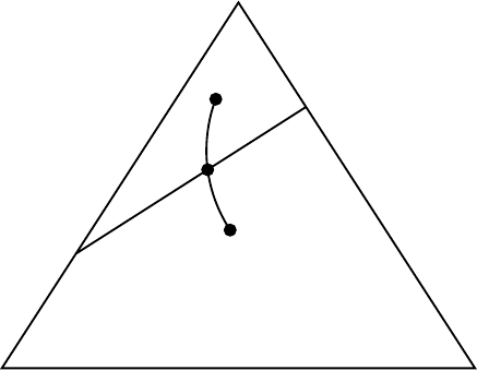
386 INFORMATION THEORY AND STATISTICS

FIGURE 11.10. Probability simplex and Chernoff information.

in A that is closest to P

; it is also the distribution in A

that is closest

to P

. By Sanov’s theorem, we can calculate the associated probabilities

of error,

= P

)

= 2

−nD(P

∗

||P

)

(11.235)

and

= P

(A)

= 2

−nD(P

∗

||P

)

. (11.236)

In the Bayesian case, the overall probability of error is the weighted sum

of the two probabilities of error,

= π

−nD(P

||P

)

+ π

−nD(P

||P

)

= 2

−n min{D(P

||P

),D(P

||P

)}

(11.237)

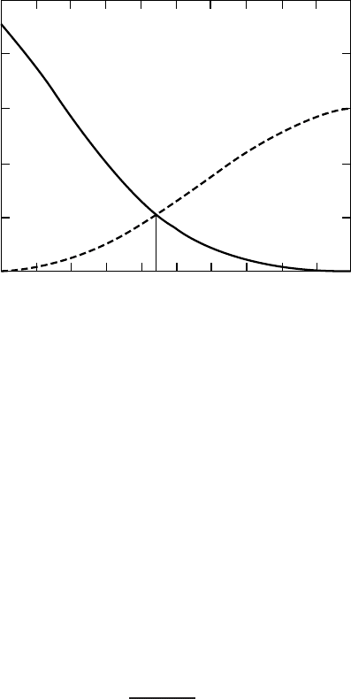
since the exponential rate is determined by the worst exponent. Since

D(P

||P

) increases with λ and D(P

||P

) decreases with λ, the maxi-

mum value of the minimum of {D(P

||P

), D(P

||P

)} is attained when

they are equal. This is illustrated in Figure 11.11. Hence, we choose λ so

that

D(P

||P

) = D(P

||P

). (11.238)

Thus, C(P

) is the highest achievable exponent for the probability of

error and is called the Chernoff information.



11.9 CHERNOFF INFORMATION 387

(

)

(

)

Relative entropy

2.5

1.5

0.5

0.1 0.2 0.3 0.4

0.5 0.6 0.7 0.8 0.9 1

FIGURE 11.11. Relative entropy D(P

||P

) and D(P

||P

) as a function of λ.

The deﬁnition D

∗

= D(P

∗

||P

) = D(P

∗

||P

) is equivalent to the

standard deﬁnition of Chernoff information,

C(P

)



=−min

0≤λ≤1

log





(x)P

1−λ

(x)



. (11.239)

It is left as an exercise to the reader to show the equivalence of (11.231)

and (11.239).

We outline brieﬂy the usual derivation of the Chernoff information

bound. The maximum a posteriori probability decision rule minimizes the

Bayesian probability of error. The decision region A for hypothesis H

for the maximum a posteriori rule is

A =



x :

(x)

> 1



, (11.240)

the set of outcomes where the a posteriori probability of hypothesis H

greater than the a posteriori probability of hypothesis H

. The probability

of error for this rule is

= π

+ π

(11.241)



(11.242)



min{π

,π

}. (11.243)

388 INFORMATION THEORY AND STATISTICS

Now for any two positive numbers a and b,wehave

min{a, b}≤a

1−λ

for all 0 ≤ λ ≤ 1. (11.244)

Using this to continue the chain, we have



min{π

,π

} (11.245)

≤



(π

)

(π

)

1−λ

(11.246)

≤



1−λ

. (11.247)

For a sequence of i.i.d. observations, P

(x) =



i=1

),and

(n)

≤



1−λ



1−λ

) (11.248)

= π

1−λ





1−λ

) (11.249)

≤





1−λ

(11.250)





1−λ



, (11.251)

where (11.250) follows since π

≤ 1,π

≤ 1. Hence, we have

log P

(n)

≤ log



(x)P

1−λ

(x). (11.252)

Since this is true for all λ, we can take the minimum over 0 ≤ λ ≤ 1,

resulting in the Chernoff information bound. This proves that the exponent

is no better than C(P

). Achievability follows from Theorem 11.9.1.

Note that the Bayesian error exponent does not depend on the actual

value of π

and π

, as long as they are nonzero. Essentially, the effect of

the prior is washed out for large sample sizes. The optimum decision rule

is to choose the hypothesis with the maximum a posteriori probability,

which corresponds to the test

,...,X

)

,...,X

)

< 1. (11.253)

11.9 CHERNOFF INFORMATION 389

Taking the log and dividing by n, this test can be rewritten as

log



log

)

> 0, (11.254)

where the second term tends to D(P

||P

) or −D(P

||P

) accordingly as

or P

is the true distribution. The ﬁrst term tends to 0, and the effect

of the prior distribution washes out.

Finally, to round off our discussion of large deviation theory and hypoth-

esis testing, we consider an example of the conditional limit theorem.

Example 11.9.1 Suppose that major league baseball players have a bat-

ting average of 260 with a standard deviation of 15 and suppose that

minor league ballplayers have a batting average of 240 with a standard

deviation of 15. A group of 100 ballplayers from one of the leagues (the

league is chosen at random) are found to have a group batting average

greater than 250 and are therefore judged to be major leaguers. We are

now told that we are mistaken; these players are minor leaguers. What

can we say about the distribution of batting averages among these 100

players? The conditional limit theorem can be used to show that the dis-

tribution of batting averages among these players will have a mean of 250

and a standard deviation of 15. To see this, we abstract the problem as

follows.

Let us consider an example of testing between two Gaussian distribu-

tions, f

= N(1,σ

) and f

= N(−1,σ

), with different means and the

same variance. As discussed in Section 11.8, the likelihood ratio test in

this case is equivalent to comparing the sample mean with a threshold.

The Bayes test is “Accept the hypothesis f = f



i=1

> 0.” Now

assume that we make an error of the ﬁrst kind (we say that f = f

when

indeed f = f

) in this test. What is the conditional distribution of the

samples given that we have made an error?

We might guess at various possibilities:

•

The sample will look like a (

) mix of the two normal distributions.

Plausible as this is, it is incorrect.

•

≈ 0foralli. This is quite clearly very unlikely, although it is

conditionally likely that

is close to 0.

•

The correct answer is given by the conditional limit theorem. If the

true distribution is f

and the sample type is in the set A, the condi-

tional distribution is close to f

∗

, the distribution in A that is closest to

. By symmetry, this corresponds to λ =

in (11.232). Calculating

390 INFORMATION THEORY AND STATISTICS

the distribution, we get

∗

(x) =



√

2πσ

−

(x−1)

2σ





√

2πσ

−

(x+1)

2σ







√

2πσ

−

(x−1)

2σ





√

2πσ

−

(x+1)

2σ



(11.255)

√

2πσ

−

+1)

2σ



√

2πσ

−

+1)

2σ

(11.256)

√

2πσ

−

2σ

(11.257)

= N (0,σ

). (11.258)

It is interesting to note that the conditional distribution is normal with

mean 0 and with the same variance as the original distributions. This

is strange but true; if we mistake a normal population for another, the

“shape” of this population still looks normal with the same variance

and a different mean. Apparently, this rare event does not result from

bizarre-looking data.

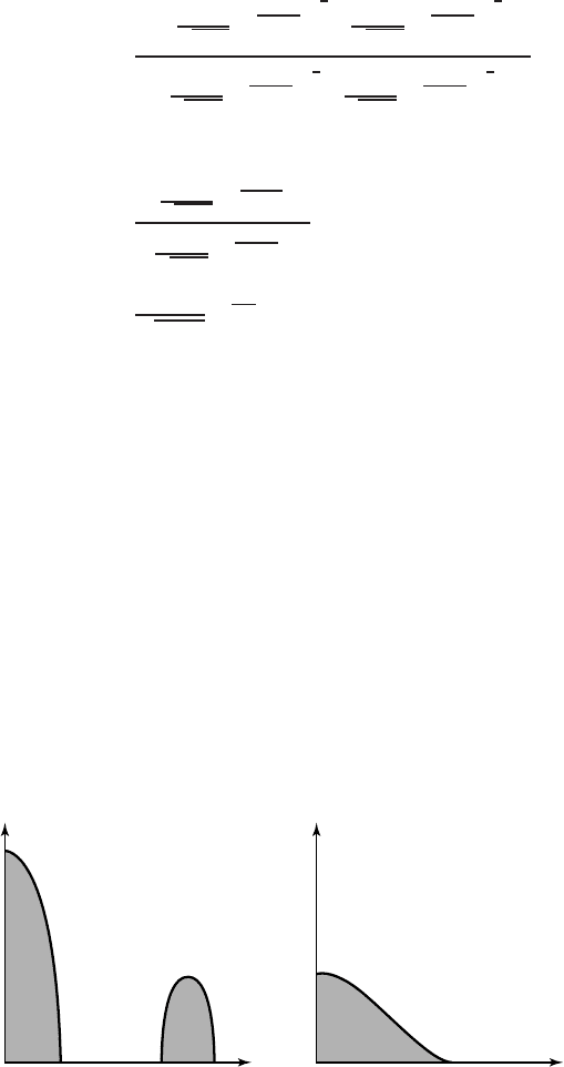
Example 11.9.2 (Large deviation theory and football ) Consider a very

simple version of football in which the score is directly related to the

number of yards gained. Assume that the coach has a choice between two

strategies: running or passing. Associated with each strategy is a distri-

bution on the number of yards gained. For example, in general, running

Yards gained in pass

Probability density

Yards gained in run

Probability density

FIGURE 11.12. Distribution of yards gained in a run or a pass play.

11.9 CHERNOFF INFORMATION 391

results in a gain of a few yards with very high probability, whereas passing

results in huge gains with low probability. Examples of the distributions

are illustrated in Figure 11.12.

At the beginning of the game, the coach uses the strategy that promises

the greatest expected gain. Now assume that we are in the closing min-

utes of the game and one of the teams is leading by a large margin.

(Let us ignore ﬁrst downs and adaptable defenses.) So the trailing team

will win only if it is very lucky. If luck is required to win, we might

as well assume that we will be lucky and play accordingly. What is the

appropriate strategy?

Assume that the team has only n plays left and it must gain l yards,

where l is much larger than n times the expected gain under each play. The

probability that the team succeeds in achieving l yards is exponentially

small; hence, we can use the large deviation results and Sanov’s theorem to

calculate the probability of this event. To be precise, we wish to calculate

the probability that



i=1

≥ nα,whereZ

are independent random

variables and Z

has a distribution corresponding to the strategy chosen.

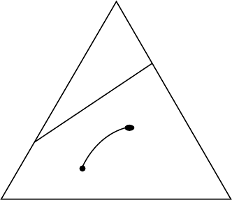
The situation is illustrated in Figure 11.13. Let E be the set of types

corresponding to the constraint,

E =



P :



a∈X

P(a)a ≥ α



. (11.259)

If P

is the distribution corresponding to passing all the time, the proba-

bility of winning is the probability that the sample type is in E,whichby

Sanov’s theorem is 2

−nD(P

∗

||P

)

,whereP

∗

is the distribution in E that is

closest to P

. Similarly, if the coach uses the running game all the time,

FIGURE 11.13. Probability simplex for a football game.

392 INFORMATION THEORY AND STATISTICS

the probability of winning is 2

−nD(P

∗

||P

)

. What if he uses a mixture of

strategies? Is it possible that 2

−nD(P

∗

||P

)

, the probability of winning with

a mixed strategy, P

= λP

+ (1 − λ)P

, is better than the probability of

winning with either pure passing or pure running? The somewhat surpris-

ing answer is yes, as can be shown by example. This provides a reason

to use a mixed strategy other than the fact that it confuses the defense.

We end this section with another inequality due to Chernoff, which

is a special version of Markov’s inequality. This inequality is called the

Chernoff bound.

Lemma 11.9.1 Let Y be any random variable and let ψ(s) be the

moment generating function of Y ,

ψ(s) = Ee

. (11.260)

Then for all s ≥ 0,

Pr(Y ≥ a) ≤ e

−sa

ψ(s), (11.261)

and thus

Pr(Y ≥ a) ≤ min

s≥0

−sa

ψ(s). (11.262)

Proof: Apply Markov’s inequality to the nonnegative random variable

. 

11.10 FISHER INFORMATION AND THE CRAM

ER–RAO

INEQUALITY

A standard problem in statistical estimation is to determine the parameters

of a distribution from a sample of data drawn from that distribution.

For example, let X

,...,X

be drawn i.i.d. ∼ N(θ, 1). Suppose that

we wish to estimate θ from a sample of size n. There are a number of

functions of the data that we can use to estimate θ . For example, we can

use the ﬁrst sample X

. Although the expected value of X

is θ , it is clear

that we can do better by using more of the data. We guess that the best

estimate of θ is the sample mean



. Indeed, it can be shown

that

is the minimum mean-squared-error unbiased estimator.

We begin with a few deﬁnitions. Let {f(x;θ)},θ∈ , denote an

indexed family of densities, f(x;θ) ≥ 0,



f(x;θ)dx = 1forallθ ∈ .

Here  is called the parameter set.

Deﬁnition An estimator for θ for sample size n is a function T :

→ .

11.10 FISHER INFORMATION AND THE CRAM

ER–RAO INEQUALITY 393

An estimator is meant to approximate the value of the parameter. It

is therefore desirable to have some idea of the goodness of the approxi-

mation. We will call the difference T − θ the error of the estimator. The

error is a random variable.

Deﬁnition The bias of an estimator T(X

,...,X

) for the param-

eter θ is the expected value of the error of the estimator [i.e., the bias is

T(x

,...,x

) − θ]. The subscript θ means that the expectation is

with respect to the density f(·;θ). The estimator is said to be unbiased

if the bias is zero for all θ ∈  (i.e., the expected value of the estimator

is equal to the parameter).

Example 11.10.1 Let X

,...,X

drawn i.i.d. ∼ f(x) = (1/λ)

−x/λ

,x ≥ 0 be a sequence of exponentially distributed random variables.

Estimators of λ include X

and X

. Both estimators are unbiased.

The bias is the expected value of the error, and the fact that it is

zero does not guarantee that the error is low with high probability. We

need to look at some loss function of the error; the most commonly

chosen loss function is the expected square of the error. A good estima-

tor should have a low expected squared error and should have an error

that approaches 0 as the sample size goes to inﬁnity. This motivates the

following deﬁnition:

Deﬁnition An estimator T(X

,...,X

) for θ is said to be consis-

tent in probability if

T(X

,...,X

) → θ in probability as n →∞.

Consistency is a desirable asymptotic property, but we are interested in

the behavior for small sample sizes as well. We can then rank estimators

on the basis of their mean-squared error.

Deﬁnition An estimator T

,...,X

) is said to dominate

another estimator T

,...,X

) if, for all θ,

(

,...,X

) − θ

)

≤ E

(

,...,X

) − θ

)

(11.263)

This raises a natural question: Is there a best estimator of θ that dom-

inates every other estimator? To answer this question, we derive the

Cram

er–Rao lower bound on the mean-squared error of any estimator.

We ﬁrst deﬁne the score function of the distribution f(x;θ).Wethenuse

the Cauchy–Schwarz inequality to prove the Cram

er–Rao lower bound

on the variance of all unbiased estimators.

394 INFORMATION THEORY AND STATISTICS

Deﬁnition The score V is a random variable deﬁned by

V =

∂

∂θ

ln f(X;θ) =

∂

∂θ

f(X;θ)

, (11.264)

where X ∼ f(x;θ).

The mean value of the score is

EV =



∂

∂θ

f(x;θ)

f(x;θ) dx (11.265)



∂

∂θ

f(x;θ) dx (11.266)

∂

∂θ



f(x;θ) dx (11.267)

∂

∂θ

1 (11.268)

= 0, (11.269)

and therefore EV

= var(V ). The variance of the score has a special

signiﬁcance.

Deﬁnition The Fisher information J(θ) is the variance of the score:

J(θ) = E



∂

∂θ

ln f(X;θ)



. (11.270)

If we consider a sample of n random variables X

,...,X

drawn

i.i.d. ∼ f(x;θ),wehave

f(x

,...,x

;θ) =



i=1

f(x

;θ), (11.271)

and the score function is the sum of the individual score functions,

V(X

,...,X

) =

∂

∂θ

ln f(X

,...,X

;θ) (11.272)



i=1

∂

∂θ

ln f(X

;θ) (11.273)



i=1

V(X

), (11.274)