Thomas M. Cover, Joy A. Thomas. Elements of information theory

Подождите немного. Документ загружается.

12.4 SPECTRUM ESTIMATION 415

This example shows that the maximum entropy may only be -achiev-

able.

12.4 SPECTRUM ESTIMATION

Given a stationary zero-mean stochastic process {X

}, we deﬁne the auto-

correlation function as

R(k) = EX

i+k

. (12.33)

The Fourier transform of the autocorrelation function for a zero-mean

process is the power spectral density S(λ):

S(λ) =

∞



m=−∞

R(m)e

−imλ

, −π<λ≤ π, (12.34)

where i =

√

−1. Since the power spectral density is indicative of the

structure of the process, it is useful to form an estimate from a sample of

the process.

There are many methods to estimate the power spectrum. The simplest

way is to estimate the autocorrelation function by taking sample averages

for a sample of length n,

R(k) =

n − k

n−k



i=1

i+k

. (12.35)

If we use all the values of the sample correlation function

R(·) to cal-

culate the spectrum, the estimate that we obtain from (12.34) does not

converge to the true power spectrum for large n. Hence, this method, the

periodogram method, is rarely used. One of the reasons for the problem

with the periodogram method is that the estimates of the autocorrelation

function from the data have different accuracies. The estimates for low

values of k (called the lags) are based on a large number of samples and

those for high k on very few samples. So the estimates are more accurate

at low k. The method can be modiﬁed so that it depends only on the

autocorrelations at low k by setting the higher lag autocorrelations to 0.

However, this introduces some artifacts because of the sudden transition to

zero autocorrelation. Various windowing schemes have been suggested to

smooth out the transition. However, windowing reduces spectral resolution

and can give rise to negative power spectral estimates.

In the late 1960s, while working on the problem of spectral estimation for

geophysical applications, Burg suggested an alternative method. Instead of

416 MAXIMUM ENTROPY

setting the autocorrelations at high lags to zero, he set them to values that

make the fewest assumptions about the data (i.e., values that maximize the

entropy rate of the process). This is consistent with the maximum entropy

principle as articulated by Jaynes [294]. Burg assumed the process to be

stationary and Gaussian and found that the process which maximizes the

entropy subject to the correlation constraints is an autoregressive Gaussian

process of the appropriate order. In some applications where we can assume

an underlying autoregressive model for the data, this method has proved

useful in determining the parameters of the model (e.g., linear predictive

coding for speech). This method (known as the maximum entropy method

or Burg’s method) is a popular method for estimation of spectral densities.

We prove Burg’s theorem in Section 12.6.

12.5 ENTROPY RATES OF A GAUSSIAN PROCESS

In Chapter 8 we deﬁned the differential entropy of a continuous random

variable. We can now extend the deﬁnition of entropy rates to real-valued

stochastic processes.

Deﬁnition The differential entropy rate of a stochastic process {X

},X

∈

R,isdeﬁnedtobe

X) = lim

n→∞

h(X

,...,X

)

(12.36)

if the limit exists.

Just as in the discrete case, we can show that the limit exists for sta-

tionary processes and that the limit is given by the two expressions

X) = lim

n→∞

h(X

,...,X

)

(12.37)

= lim

n→∞

h(X

n−1

,...,X

). (12.38)

For a stationary Gaussian stochastic process, we have

h(X

,...,X

) =

log(2πe)

(n)

|, (12.39)

where the covariance matrix K

(n)

is Toeplitz with entries R(0), R(1),...,

R(n − 1) along the top row. Thus, K

(n)

= R(i − j) = E(X

− EX

)(X

12.6 BURG’S MAXIMUM ENTROPY THEOREM 417

− EX

).Asn →∞, the density of the eigenvalues of the covariance

matrix tends to a limit, which is the spectrum of the stochastic process.

Indeed, Kolmogorov showed that the entropy rate of a stationary Gaussian

stochastic process can be expressed as

X) =

log 2πe +

4π



−π

log S(λ) dλ. (12.40)

The entropy rate is also lim

n→∞

h(X

n−1

). Since the stochastic pro-

cess is Gaussian, the conditional distribution is also Gaussian, and hence

the conditional entropy is

log 2πeσ

∞

,whereσ

∞

is the variance of the

error in the best estimate of X

given the inﬁnite past. Thus,

∞

2πe

2h(X )

, (12.41)

where h(

X) is given by (12.40). Hence, the entropy rate corresponds to

the minimum mean-squared error of the best estimator of a sample of the

process given the inﬁnite past.

12.6 BURG’S MAXIMUM ENTROPY THEOREM

Theorem 12.6.1 The maximum entropy rate stochastic process {X

} sat-

isfying the constraints

i+k

= α

,k= 0, 1,...,p for all i, (12.42)

is the pth-order Gauss–Markov process of the form

=−



k=1

i−k

+ Z

, (12.43)

where the Z

are i.i.d. ∼ N(0,σ

) and a

,...,a

,σ

are chosen to

satisfy (12.42).

Remark We do not assume that {X

} is (a) zero mean, (b) Gaussian, or

Proof: Let X

,...,X

be any stochastic process that satisﬁes the

constraints (12.42). Let Z

,...,Z

be a Gaussian process with the

same covariance matrix as X

,...,X

. Then since the multivariate

normal distribution maximizes the entropy over all vector-valued random

418 MAXIMUM ENTROPY

variables under a covariance constraint, we have

h(X

,...,X

) ≤ h(Z

,...,Z

) (12.44)

= h(Z

,...,Z

) +



i=p+1

h(Z

i−1

i−2

,...,Z

)

(12.45)

≤ h(Z

,...,Z

) +



i=p+1

h(Z

i−1

i−2

,...,Z

i−p

)

(12.46)

by the chain rule and the fact that conditioning reduces entropy. Now

deﬁne Z



,...,Z



as a pth-order Gauss–Markov process with the

same distribution as Z

,...,Z

for all orders up to p. (Existence of

such a process will be veriﬁed using the Yule–Walker equations immedi-

ately after the proof.) Then since h(Z

i−1

,...,Z

i−p

) depends only on

the pth-order distribution, h(Z

i−1

,...,Z

i−p

) = h(Z



i−1

,...,Z



i−p

and continuing the chain of inequalities, we obtain

h(X

,...,X

) ≤ h(Z

,...,Z

) +



i=p+1

h(Z

i−1

i−2

,...,Z

i−p

)

(12.47)

= h(Z



,...,Z



) +



i=p+1

h(Z



i−1



i−2

,...,Z



i−p

)

(12.48)

= h(Z



,...,Z



), (12.49)

where the last equality follows from the pth-order Markovity of the {Z



Dividing by n and taking the limit, we obtain

lim

h(X

,...,X

) ≤ lim

h(Z



,...,Z



) = h

∗

, (12.50)

where

∗

log 2πeσ

, (12.51)

which is the entropy rate of the Gauss–Markov process. Hence, the max-

imum entropy rate stochastic process satisfying the constraints is the

pth-order Gauss–Markov process satisfying the constraints.



A bare-bones summary of the proof is that the entropy of a ﬁnite

segment of a stochastic process is bounded above by the entropy of a

12.6 BURG’S MAXIMUM ENTROPY THEOREM 419

segment of a Gaussian random process with the same covariance structure.

This entropy is in turn bounded above by the entropy of the minimal order

Gauss–Markov process satisfying the given covariance constraints. Such

a process exists and has a convenient characterization by means of the

Yule–Walker equations given below.

Note on the choice of a

,...,a

and σ

: Given a sequence of covariances

R(0), R(1),...,R(p), does there exist a pth-order Gauss–Markov pro-

cess with these covariances? Given a process of the form (12.43), can we

choose the a

’s to satisfy the constraints? Multiplying (12.43) by X

i−l

and taking expectations, noting that R(k) = R(−k),weget

R(0) =−



k=1

R(−k) + σ

(12.52)

and

R(l) =−



k=1

R(l − k), l = 1, 2,.... (12.53)

These equations are called the Yule–Walker equations.Therearep + 1

equations in the p + 1 unknowns a

,...,a

,σ

. Therefore, we can

solve for the parameters of the process from the covariances.

Fast algorithms such as the Levinson algorithm and the Durbin algo-

rithm [433] have been devised to use the special structure of these

equations to calculate the coefﬁcients a

,...,a

efﬁciently from the

covariances. (We set a

= 1 for a consistent notation.) Not only do the

Yule–Walker equations provide a convenient set of linear equations for

calculating the a

’s and σ

from the R(k)’s, they also indicate how the

autocorrelations behave for lags greater than p. The autocorrelations for

high lags are an extension of the values for lags less than p. These val-

ues are called the Yule–Walker extension of the autocorrelations. The

spectrum of the maximum entropy process is seen to be

S(λ) =

∞



m=−∞

R(m)e

−imλ

(12.54)



1 +



k=1

−ikλ



, −π ≤ λ ≤ π. (12.55)

This is the maximum entropy spectral density subject to the constraints

R(0), R(1),...,R(p).

However, for the pth-order Gauss–Markov process, it is possible to

calculate the entropy rate directly without calculating the a

’s. Let K

420 MAXIMUM ENTROPY

the autocorrelation matrix corresponding to this process—the matrix with

,...,R

along the top row. For this process, the entropy rate is

equal to

∗

= h(X

p−1

,...,X

) = h(X

,...,X

) − h(X

,...,X

p−1

)

(12.56)

log(2πe)

p+1

|−

log(2πe)

p−1

(12.57)

log(2πe)

p−1

. (12.58)

In a practical problem, we are generally given a sample sequence

,...,X

, from which we calculate the autocorrelations. An impor-

tant question is: How many autocorrelation lags should we consider (i.e.,

what is the optimum value of p)? A logically sound method is to choose

the value of p that minimizes the total description length in a two-stage

description of the data. This method has been proposed by Rissanen

[442, 447] and Barron [33] and is closely related to the idea of Kol-

mogorov complexity.

SUMMARY

Maximum entropy distribution. Let f be a probability density satis-

fying the constraints



f(x)r

(x) = α

for 1 ≤ i ≤ m. (12.59)

Let f

∗

(x) = f

(x) = e



i=1

(x)

, x ∈ S,andletλ

,...,λ

be cho-

sen so that f

∗

satisﬁes (12.59). Then f

∗

uniquely maximizes h(f ) over

all f satisfying these constraints.

Maximum entropy spectral density estimation. The entropy rate of a

stochastic process subject to autocorrelation constraints R

,...,R

is maximized by the pth order zero-mean Gauss-Markov process satis-

fying these constraints. The maximum entropy rate is

∗

log(2πe)

p−1

, (12.60)

PROBLEMS 421

and the maximum entropy spectral density is

S(λ) =



1 +



k=1

−ikλ



. (12.61)

PROBLEMS

12.1 Maximum entropy. Find the maximum entropy density f ,

deﬁned for x ≥ 0, satisfying EX = α

,Eln X = α

. That is, max-

imize −



f ln f subject to



xf (x ) d x = α



(ln x)f(x)dx =

, where the integral is over 0 ≤ x<∞. What family of densi-

tiesisthis?

12.2 Min D(P  Q) under constraints on P . We wish to ﬁnd the

(parametric form) of the probability mass function P(x),x ∈{1, 2,

...} that minimizes the relative entropy D(P  Q) over all P such

that



P(x)g

(x) = α

,i = 1, 2,... .

(a) Use Lagrange multipliers to guess that

∗

(x) = Q(x)e



∞

i=1

(x)+λ

(12.62)

achieves this minimum if there exist λ

’s satisfying the α

constraints. This generalizes the theorem on maximum en-

tropy distributions subject to constraints.

(b) Verify that P

∗

minimizes D(P  Q).

12.3 Maximum entropy processes. Find the maximum entropy rate

stochastic process {X

}

∞

−∞

subject to the constraints:

(a) EX

= 1,i= 1, 2,....

(b) EX

= 1, EX

i+1

,i= 1, 2,....

(a) and (b).

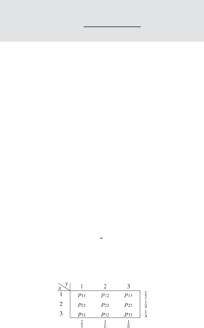
12.4 Maximum entropy with marginals. What is the maximum en-

tropy distribution p(x, y) that has the following marginals?

422 MAXIMUM ENTROPY

(Hint: You may wish to guess and verify a more general result.)

12.5 Processes with ﬁxed marginals. Consider the set of all densities

with ﬁxed pairwise marginals f

), f

),...,

n−1

). Show that the maximum entropy process with

these marginals is the ﬁrst-order (possibly time-varying) Markov

process with these marginals. Identify the maximizing f

∗

...,x

12.6 Every density is a maximum entropy density .Letf

(x) be a

given density. Given r(x),letg

(x) be the density maximizing

h(X) over all f satisfying



f (x)r(x)dx = α.Nowletr(x) =

ln f

(x). Show that g

(x) = f

(x) for an appropriate choice α =

. Thus, f

(x) is a maximum entropy density under the constraint



f ln f

= α

12.7 Mean-squared error.Let{X

}

i=1

satisfy EX

i+k

= R

,k =

0, 1,...,p. Consider linear predictors for X

;thatis,

n−1



i=1

n−i

Assume that n>p.Find

max

f(x

)

min

E(X

−

)

where the minimum is over all linear predictors b and the maxi-

mum is over all densities f satisfying R

,...,R

12.8 Maximum entropy characteristic functions. We ask for the max-

imum entropy density f(x),0 ≤ x ≤ a, satisfying a constraint on

the characteristic function (u) =



iux

f(x)dx. The answers

need be given only in parametric form.

(a) Find the maximum entropy f satisfying



f(x)cos(u

x)dx

= α, at a speciﬁed point u

(b) Find the maximum entropy f satisfying



f(x)sin(u

x)dx

= β.

given value of the characteristic function (u

) at a speciﬁed

point u

(d) What problem is encountered if a =∞?

PROBLEMS 423

12.9 Maximum entropy processes

(a) Find the maximum entropy rate binary stochastic process

}

∞

i=−∞

∈{0, 1}, satisfying Pr{X

= X

i+1

for

all i.

(b) What is the resulting entropy rate?

12.10 Maximum entropy of sums.LetY = X

+ X

. Find the maxi-

mum entropy density for Y under the constraint EX

= P

, EX

= P

(a) If X

and X

are independent.

(b) If X

and X

are allowed to be dependent.

12.11 Maximum entropy Markov chain.Let{X

} be a stationary

Markov chain with X

∈{1, 2, 3}.LetI(X

n+2

) = 0foralln.

(a) What is the maximum entropy rate process satisfying this

constraint?

(b) What if I(X

n+2

) = α for all n for some given value of

α,0≤ α ≤ log 3?

12.12 Entropy bound on prediction error.Let{X

} be an arbitrary real

valued stochastic process. Let

n+1

= E{X

n+1

}. Thus the con-

ditional mean

n+1

is a random variable depending on the n-past

.Here

n+1

is the minimum mean squared error prediction of

n+1

given the past.

(a) Find a lower bound on the conditional variance E{E{(X

n+1

−

n+1

)

}} in terms of the conditional differential entropy

h(X

n+1

(b) Is equality achieved when {X

} is a Gaussian stochastic pro-

cess?

12.13 Maximum entropy rate. What is the maximum entropy rate sto-

chastic process {X

} over the symbol set {0, 1} for which the

probability that 00 occurs in a sequence is zero?

12.14 Maximum entropy

(a) What is the parametric-form maximum entropy density f(x)

satisfying the two conditions

= a, EX

= b?

(b) What is the maximum entropy density satisfying the condition

E(X

+ X

) = a + b?

424 MAXIMUM ENTROPY

12.15 Maximum entropy. Find the parametric form of the maximum

entropy density f satisfying the Laplace transform condition



f(x)e

−x

dx = α,

and give the constraints on the parameter.

12.16 Maximum entropy processes. Consider the set of all stochastic

processes with {X

},X

∈ R, with

= EX

= 1,R

= EX

i+1

Find the maximum entropy rate.

12.17 Binary maximum entropy. Consider a binary process {X

},X

∈

{−1, +1}, with R

= EX

= 1andR

= EX

i+1

(a) Find the maximum entropy process with these constraints.

(b) What is the entropy rate?

12.18 Maximum entropy. Maximize h(Z, V

) subject to the en-

ergy constraint E(

mV 

+ mgZ) = E

. Show that the resulting

distribution yields

mV 

,EmgZ=

Thus,

of the energy is stored in the potential ﬁeld, regardless of

its strength g.

12.19 Maximum entropy discrete processes

(a) Find the maximum entropy rate binary stochastic process

}

∞

i=−∞

∈{0, 1}, satisfying Pr{X

= X

i+1

for all

(b) What is the resulting entropy rate?

12.20 Maximum entropy of sums.LetY = X

+ X

. Find the maxi-

mum entropy of Y under the constraint EX

= P

,EX

= P

(a) If X

and X

are independent.

(b) If X

and X

are allowed to be dependent.