Tsoulos George (ред.) MIMO System Technology for Wireless Communications

Подождите немного. Документ загружается.

184 MIMO System Technology for Wireless Communications

different goals: allocate equal power to all users, allocate equal capacity to

all users, or maximize sum capacity. Sum capacity can be maximized by

computing the gain of each of the independent channels and using the water-

ﬁlling algorithm to distribute the available power.

A very simple way of allocating the power is to set , = LI, where L = 1/W.

One problem with channel inversion arises when H is ill-conditioned. In

such cases, at least one of the singular values of is very large, L will

be large, and the SNR at the receivers will be low. It is interesting to note

the similarity between channel inversion and least-squares or “zero-forcing”

(ZF) receive beamforming, which applies a dual of the transformation in

Equation 7.4 to the receive data. Such beamformers are known to cause noise

ampliﬁcation when the channel is nearly rank deﬁcient. On the transmit side,

ZF produces signal attenuation instead. In fact, it has been shown that in

the ideal case where the elements of H are independent complex Gaussian

random variables, the probability density of L has an inﬁnite mean [17]. It

is also shown in [17] and the simulation results section of this chapter that

the capacity of channel inversion does not grow linearly with K.

7.3.1.2 Regularized Channel Inversion

When rank-deﬁcient channels are encountered in ZF receive beamforming,

one technique to reduce the effects of noise ampliﬁcation is to regularize the

inverse in the ZF ﬁlter. If the noise is spatially white and an appropriate

regularization value is chosen, this approach is equivalent to using a mini-

mum mean-squared error (MMSE) criterion to design the beamformer

weights. Applying this principle to the transmit side suggests the following

solution:

(7.5)

where _ is the regularization parameter. When _ | 0, the transmitter does

not perfectly cancel out all interference. The key is to deﬁne a value for _

that optimally trades off the numerical condition of the matrix inverse

against the amount of interference that is produced. It has been shown that

choosing _ = K/W approximately maximizes the SINR at each receiver, and

leads to linear capacity growth with K [17]. Because each user sees some

interference from other users, this scheme does not allow the same ﬂexibility

as exact channel inversion in adjusting the power transmitted to each user,

because a change to the power weighting for one user changes the interfer-

ence seen by all other users.

7.3.1.3 Optimal Linear Precoders

Regularized channel inversion demonstrates that perfectly canceling out all

inter-user interference is not optimal, and provides a good solution in closed

()HH

1

HH I

()







4190_book.fm Page 184 Tuesday, February 21, 2006 9:14 AM

Performance of Multi-User Spatial Multiplexing with Measured Channel Data 185

form at low computational cost. However, it is still not necessarily the optimal

linear beamformer. Attempting to design a set of transmit beamformers with-

out any constraints on inter-user interference is a very challenging problem

because they are all interdependent. If an optimal beamformer is designed

for one user, it will produce some interference for the other users. If the

interference is taken into account in designing an optimal beamformer for a

second user, it will emit interference that makes the ﬁrst user’s beamformer

suboptimal. This suggests that the optimal solution can not be computed in

closed form but requires an iterative approach.

With a zero-forcing solution, a set of independent channels is created, so

the power transmitted to each user can readily be adjusted to achieve a

variety of different goals, such as maximizing sum capacity or insuring equal

capacity for all users given a power constraint, or minimizing power given

a capacity constraint for each user. In the case where inter-user interference

is allowed, the solution to each of these problems will be different. Optimal

transmit beamformers have been found for a variety of different optimization

criteria [18–23]. We give as an example the linear precoder that optimizes

sum capacity [18], which takes the form

(7.6)

This is similar to regularized channel inversion, but we have introduced

two diagonal matrices, D and ), which are used respectively to weight the

rows of H inside the inverse and weight the columns of the resulting beam-

former. The optimal values for these matrices, and the scale constant _, can

be computed using the iterative algorithm given in Table 7.1.

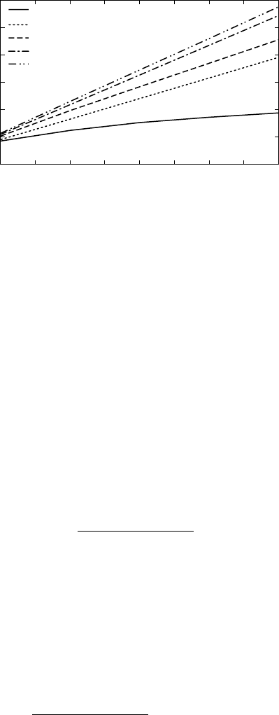
The sum capacity as a function of the channel matrix size for the linear

precoders we have discussed so far is compared with the sum capacity of

the channel and capacity of an equivalent single-user channel in Figure 7.4.

TABLE 7.1

Linear Precoding for Maximum Sum Capacity

1. Initialize W

(1) = 1 for j = 1…K, D = I, ) = I

2. Repeat until convergence

sHDHI Hd=+ ) .





MHDH DIH=+

()

)



tr( )/W

WHM MM=



W/tr( )

jjj

[]W

iij

=,|

[]W

[]

()

jj j

dd n

[] [ ]) =

,,jj jj j

dW /

4190_book.fm Page 185 Tuesday, February 21, 2006 9:14 AM

186 MIMO System Technology for Wireless Communications

Of all the precoders, only channel inversion fails to achieve a sum capacity

that increases linearly with K and n

. Regularized channel inversion offers

a substantial improvement in performance, and the optimal linear precoder

(labeled capacity-optimal RCI) is even better, achieving most of the sum-

capacity of the channel that is achievable using DPC.

As we noted earlier, there are many situations in which optimizing sum

capacity is problematic because it does not guarantee a minimum level of

signal to any user. There are many other optimizations that have appeared

recently in the literature that may be of greater practical interest. The “power

control” problem was the ﬁrst of these [19,20], and can be stated as follows:

given a set of SINR requirements for each user, compute the set of beam-

formers b

, …, b

such that the SINR requirements are met and total trans-

mitted power is minimized. We deﬁne L

as the SINR for user j, which can

be expressed as:

(7.7)

where we have assumed that the noise has unit variance. The power mini-

mization problem can be stated mathematically as

(7.8)

FIGURE 7.4

Mean sum-capacity of various precoders for uncorrelated Gaussian channels with K users and

= K transmitters at a SNR of 10 dB.

10 9 8 7 6 5 4 3 2

Capacity(bits/usr)

Channel inversion

Regularized channel inversion

Capacity-optimal RCI

Sum capacity

Single user

jjjj

kjjk



bHHb

bHHb 1

min





bbHHb

bHHb

jjjj

kjjk



v =,.

1L ,,

4190_book.fm Page 186 Tuesday, February 21, 2006 9:14 AM

Performance of Multi-User Spatial Multiplexing with Measured Channel Data 187

Solutions to this problem have been proposed in [19–21]. Other optimizations

for which solutions have recently been proposed include the maximization of

the SINR margin for all users given a minimum SINR requirement for each

user and a total power constraint [22,23]. In addition to the sum-capacity solu-

tion, [18] also proposes a solution for maximizing the minimum capacity for

each of the individual users. This whole class of solutions requires more

computation than plain or regularized inversion, but since beamformers are

typically computed once for an entire block of transmitted symbols, this is

still a practical solution.

7.3.2 Linear Processing, Multi-Antenna Receivers

With only a single antenna, the receivers are not able to perform spatial

interference suppression of their own, so they can only receive data over a

single spatial channel. With multiple antennas, these restrictions are

removed, provided that the transmitter and receiver can coordinate their

spatial processing, and appropriately allocate the available spatial resources.

A simple approach to this would be to apply the single-antenna techniques

just described, provided that n

f n

, where n

is the total number of receive

antennas summed over all users. This effectively treats each receive antenna

as if it were a separate user, so no joint processing among the receive antennas

is required, but performance is limited because the problem is overly con-

strained, and the number of users is limited more than necessary.

Both channel inversion and regularized channel inversion limit the num-

ber of users to K f n

. For optimal beamforming, it is technically possible to

support cases where K > n

, but realistically this can occur only when the SINR

requirements are very low. So, it is reasonable to consider n

to be the

practical upper bound on the number of users. If the receivers have multiple

antennas, it is still possible to support up to K = n

users by using the concept

of coordinated beamforming. To illustrate this, consider the block diagram

of Figure 7.2. Assume that the decoding function for user j is a linear

operator w

, so that

= . If the beamformers were known to the trans-

mitter in advance, then the virtual channel, which represents the transfer

function from the transmitter to the output of the beamformer of user j, is

If we collect the virtual channels for each user, we can deﬁne a virtual

channel for the entire system:

As long as K f n

, it possible to apply any of the single-antenna algorithms

described earlier to the virtual channel . The remaining problem is deter-

mining the receive beamformers w

. This information could be obtained if

()



hwH

jjj



H= h h … h

12 K

4190_book.fm Page 187 Tuesday, February 21, 2006 9:14 AM

188 MIMO System Technology for Wireless Communications

the transmitter were to assume a speciﬁc approach to designing the beam-

formers. For example, both MMSE and MRC designs for w

are functions of

only the channel and the transmit beamformers, so w

could be computed

from information available to the transmitter. However, this results in a

situation where the solutions to the transmit and receive beamformers are

dependent on each other. This suggests the following iterative approach:

1. Assume an initial set of w

values.

2. Compute the virtual channel and the transmit beamformers.

3. Update the receive beamformers w

4. Repeat steps 2 and 3 until convergence.

The convergence properties of this approach will depend, in general, on

what algorithms are used on both the transmitter and receiver side to determine

the beamforming weights. The concept of beamforming that is coordinated

between the transmitter and receiver is the basis for several recent multi-

user transmission schemes [1,24–29].

In single-user MIMO channels with CSI available to the transmitter, capacity

is achieved by spatial multiplexing, where a number of independent sub-

channels are created that carry independent streams of data. In a multi-user

MIMO downlink where the receivers have multiple antennas, it is also pos-

sible to transmit multiple data streams to each user. We deﬁne m

to be the

number of sub-channels allocated to user j, and

to be the total number of sub-channels. The restrictions on these values are

that m

, where

is the rank of and m f n

This means that allocating multiple sub-channels to individual users limits

the total number of users that can be served. The problem of choosing a

good value of m

has not yet been studied extensively, but the simulation

results presented later in this chapter illustrate the trade-offs involved. In

the case where m

> 1, deﬁne the receiver for user j as the m

× n

matrix W

and the linear precoder as the n

× m matrix,

where B

is the n

× m

precoder for user j. As in the single sub-channel case,

the transmit precoders B

can be derived by selecting an initial set of receivers

, and alternately updating B

and W

until convergence is reached.

In this section, we discuss two general approaches to this problem. The

ﬁrst is a coordinated zero-forcing approach that is a generalization of channel



……HH HH H

 +111

B =

BB B

…

4190_book.fm Page 188 Tuesday, February 21, 2006 9:14 AM

Performance of Multi-User Spatial Multiplexing with Measured Channel Data 189

inversion. The second is a framework for applying other methods like reg-

ularized channel inversion or optimal beamforming in a context where users

have multiple antennas.

7.3.2.1 Coordinated Zero-Forcing

As noted previously, in cases where the receivers have multiple antennas, it

is possible to use channel inversion at the transmitter if n

f n

, but this over-

constrains the problem, by forcing HB to be completely diagonal. In fact, all

inter-user interference can be eliminated by constraining HB to be block-

diagonal (i.e., H

= 0, for i | j). A procedure for computing the optimal B

given this constraint has been proposed [24,30–34], but it imposes restrictions

on the channel conﬁgurations that can be accommodated. In order to accom-

modate all possible receiver sizes, those restrictions can be eliminated using

the coordinated beamforming approach: estimate the receivers W

and force

to be zero. A method for computing this iteratively, referred to as

the “coordinated zero-forcing” algorithm, is listed in Table 7.2.

TABLE 7.2

Coordinated Zero-Forcing Algorithm

1. For each user, initialize W

as the m

dominant left singular vectors of H

, and deﬁne H

–

2. For each user, deﬁne

let represent an orthogonal basis for the right null space of and compute the SVD

where and represent the ﬁrst m

left and right singular vectors. Update the

transmitter and receiver beamformers: and and deﬁne

3. Repeat step 2 until

for some value of J.

4. Use water-ﬁlling to determine power allocation given the diagonal values of the 8

matrices as the channel gains.

WHB

iij





HH HH H

=… …

 +111



()0



UU VV

()





½½

()1

()

BB=







min

[]

=,,

4190_book.fm Page 189 Tuesday, February 21, 2006 9:14 AM

190 MIMO System Technology for Wireless Communications

The result of the coordinated zero-forcing algorithm is a set of non-inter-

fering virtual channels. One advantage of this approach is that, since the

channels do not interfere, the solution is independent of the power allocation

to each channel, and therefore the power allocation can be performed inde-

pendently from the computation of the beamformers.

There are a few special cases of the coordinated zero-forcing algorithm

worth noting. First, if n

= 1 for all users, the solution is equivalent to channel

inversion with optimal power allocation. Second, if n

> max{rank(H

…,

rank(H

)},

the convergence criterion is reached at the ﬁrst step, and the solution

is equivalent to the block-diagonalization solution of [24]. Third, if m

= 1 for

all users, the receiver beamformers W

are equivalent to maximal ratio combin-

ers, and the solution for B is equivalent to channel inversion of H

–

(this allows

for some computational savings over the generalized implementation).

7.3.2.2 General Coordinated Beamforming

As noted in the discussion of channel inversion, the use of zero-forcing at

the transmitter has some disadvantages, so there are good reasons to use

other beamforming methods at the transmitter. This can be done in channels

where the receivers have multiple antennas by applying the same general

approach as in coordinated zero-forcing. A general algorithm for doing this

is listed in Table 7.3.

There are two reasons that computing the zero-forcing solution makes a good

initialization point for the algorithm in step 1. The ﬁrst is that as SNR increases,

the difference between the zero-forcing solution and other beamforming algo-

rithms will become increasingly small, so starting with the zero-forcing

solution can signiﬁcantly reduce the number of iterations to convergence

[29]. The second reason is that zero-forcing is the only way the beamforming

weights and power allocation can be decided independently, so initializing

with zero-forcing is a means of intelligently estimating how many bits should

be allocated to each sub-channel before proceeding with beamformer opti-

mization. In [29] this approach was used with MMSE receivers and optimal

beamforming for minimum power at the transmitter.

TABLE 7.3

Coordinated Transmitter/Receiver Beamforming Algorithm

1. Assume an initial set of receiver weights W

, …, W

. Two good candidates for this are

to use the dominant left singular vectors of the respective channel matrices H

, or to

compute the full coordinated zero-forcing solution and use the resulting values of W

2. Given W

, …, W

, calculate

–

H and ﬁnd B using any of the algorithms discussed earlier

(regularized channel inversion, optimal beamforming).

3. Given B, recalculate the receiver beamformers W

, …, W

according to some assumed

receiver design (MMSE, MRC, etc).

4. If the SNR or sum rate achieved by B and w

has changed from the last iteration, go to

step 2; otherwise, stop.

4190_book.fm Page 190 Tuesday, February 21, 2006 9:14 AM

Performance of Multi-User Spatial Multiplexing with Measured Channel Data 191

7.3.3 Non-Linear Processing Methods

All of the transmission schemes discussed so far use linear processing at the

transmitter and receiver. However, as noted previously, channel capacity in

a multi-user environment depends on the use of DPC techniques, which are

inherently non-linear in nature. DPC techniques have been demonstrated to

outperform linear methods [13], but implementation is more expensive.

Some efﬁcient DPC precoders have computational complexity similar to that

of linear precoders, but the computation must be performed separately for

each transmitted symbol, while linear precoders can be computed once for an

entire block of transmitted symbols.

Another limitation of DPC it that none yet exists that is designed for

multiple-antenna receivers. However, there are straightforward ways of

combining DPC with linear processing methods to make them usable for

multi-antenna receivers. One simple example is using coordinated zero-

forcing to compute a set of transmit and receive vectors that allow one sub-

channel per user (m

= 1). After this is computed, the linear beamformers

could be replaced by a DPC encoder that uses the channel matrix .

It is reasonable to assume that in a real multi-user environment it will be

common to have a mixture of users with single and multiple antennas. In

this type of environment, one proposal for obtaining the beneﬁts of non-

linear precoding is to use block-diagonalization for the users with multiple

antennas and non-linear DPC methods for the users with only one antenna

[35]. In this approach, the beamformers for the multiple-antenna users are

chosen to lie in the null space of the channel matrices of the other users

including those with single antennas. The equivalent channel for the single-

antenna users looks as if there are no multiple-antenna users present, which

improves diversity for those users. The data transmitted to the multiple-

antenna users are also precoded using a linear precoder in order to eliminate

the multi-user interference, which in this case only originates from the single-

antenna users. This approach signiﬁcantly improves the performance of the

single-antenna users and, hence, also that of the overall system.

7.4 Channel Measurements

In the results that follow, we examine the performance of linear precoding

schemes in realistic environments using channel measurements from both

indoor and outdoor propagation environments. The measurements were

taken from a narrowband channel sounding system designed and built at

Brigham Young University (BYU). The transmitter of the system modulates

the chosen carrier frequency using BPSK modulation with a unique pseudo-

random binary sequence for each of the antennas in the transmit array. In

the receiver, the signals from each of the elements of the receive array are

4190_book.fm Page 191 Tuesday, February 21, 2006 9:14 AM

192 MIMO System Technology for Wireless Communications

down-converted to an intermediate frequency and sampled using a high

frequency, multi-channel, analog-to-digital converter. The sampled signals

are stored and processed off-line to extract the complex gain from each of

the transmit antennas to each of the receive antennas. The frequency with

which the channel can be sampled is a function of the length of binary

sequence used for modulation. For a more detailed description of the channel

sounder and the post-processing, see [36].

All of the results included here were collected at a carrier frequency of

2.43 GHz, with a bandwidth of 25 KHz. This frequency is used by some of

the popular wireless LAN standards and is close to the 1.9 GHz frequency

used in some mobile telephone networks. In the measurement results pre-

sented here, the transmitter was kept at a ﬁxed location and the receiver

moved while sampling the channel every 2.5 ms. Multi-user channels are

created by selecting samples from multiple points along the measurement

path. Because the average number of samples per wavelength is as high as

30 for most of the cases considered here, relatively small separations between

users can be simulated.

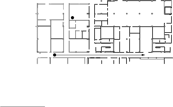
The measurements used here come from three different sets. The ﬁrst is a

set of indoor measurements taken inside a typical university building.* The

measurements were taken with the transmitter in a ﬁxed location and the

receiver moving in a straight path with an approximate length of about

40 meters along a long corridor at constant speed. The measurement path is

illustrated in Figure 7.5. All channels were non-line-of-sight (NLOS), which

would typically lead to reduced power but enhanced multipath diversity

relative to line-of-sight (LOS) channels. Both the transmitter and receiver

used 10 monopole antennas arranged in a circular pattern with a radius of

0.86 wavelengths, equivalent to a spacing of approximately 0.5 wavelengths

between adjacent elements.

* The building was the Clyde Engineering Building on the BYU campus, which has steel-rein-

forced concrete structural walls and cinder-block partition walls.

FIGURE 7.5

Illustration of the measurement path and part of the building used for the indoor channel

measurements.

Transmitter

Receiver

4190_book.fm Page 192 Tuesday, February 21, 2006 9:14 AM

Performance of Multi-User Spatial Multiplexing with Measured Channel Data 193

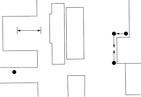
Two outdoor data sets are also considered here. The ﬁrst, referred to as

outdoor channel A, placed the transmitter between two buildings on the

BYU campus, and the receiver behind a neighboring building, creating a

NLOS channel similar to that often seen in urban environments. These meas-

urements were collected with 8-element uniform linear arrays of monopole

antennas at both transmitter and receiver, with a spacing of 0.3 wavelengths.

The receiver was placed at three different locations and moved along a

straight path with a length of about 10 meters. The measurement paths and

neighboring buildings for outdoor channel A are illustrated in Figure 7.6.

The results in the next section derived from these measurements are aver-

aged over the three different locations.

The second outdoor environment, referred to in the next section as outdoor

channel B, contained mostly LOS channels. The transmitter was placed in

two locations a few meters from the wall of a building. The receiver was

placed at four different locations near the same building, and moved dis-

tances of 10–12 meters. These measurements were collected using uniform

linear arrays of seven antennas at both transmitter and receiver with a

spacing of 0.39 wavelengths. The building and the measurement paths for

this channel are illustrated in Figure 7.7. The composite results for outdoor

channel B also are averaged over the four measurement locations.

Most of the test cases considered scenarios with fewer antennas than the

original data set. Appropriate antenna subsets were selected as follows. On the

transmit side, antennas with maximal separation were chosen to mimic a base

station that uses the entire array aperture. For example, the 4-element trans-

mitter that is used in many of the results is taken from the 7-element linear

array by choosing 4 elements with uniform separation of 0.78 wavelengths.

A mobile receiver, on the other hand, would be expected to have limited

FIGURE 7.6

Illustration of the measurement paths and neighboring buildings for outdoor channel A. These

channels are almost all non-line-of-sight (NLOS).

Location 1

Receiver

Location 2

Location 3

Transmitter

10 m

4190_book.fm Page 193 Tuesday, February 21, 2006 9:14 AM