Velten K. Mathematical Modeling and Simulation: Introduction for Scientists and Engineers
Подождите немного. Документ загружается.

4.10 A Look Beyond the Heat Equation 305
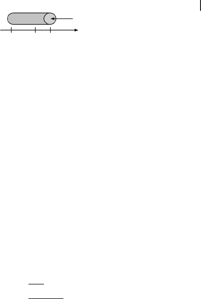
F
x
L
L −ΔL
0
Fig. 4.29 One-dimensional deformation of a cylinder.
the cylinder in terms of its strain .Inthesimplestcase,thiscanbewrittenasa
linear equation in the form of the well-known Hooke’s law:
σ = E · (4.141)
where E (Pa) is the so-called Young’s modulus of elasticity. Young’s moduli of
elasticity are listed for most relevant materials in books such as [208]. Equation
4.141 can be generalized in a number of ways [207]. In particular, you should
note that the material law typically will be nonlinear, and that will be a tensorial
quantity in general, which describes the deformed state in a direction-dependent
way similar to σ . In the case of a homogeneous, isotropic material (i.e. a material
with direction-independent properties), Hooke’s law can be written as [207]
σ = 2μ + λtr() ·I (4.142)
where σ is the stress tensor (Equation 4.137) and is the strain tensor
=
⎛
⎜
⎝
11
12
13
21
22
23
31
32
33
⎞
⎟
⎠
(4.143)
tr(), the trace of ,isdefinedas
tr() =
11
+
22
+
33
(4.144)
In Equation 4.142, μ is the shear modulus or modulus of rigidity and λ is Lame’s
constant. μ and λ describe the material properties in Equation 4.142. In many books
(such as [208]), these parameters are given in terms of Young’s modulus E and
Poisson’s ratio ν as follows [207]:
μ =
E
2 +2ν
(4.145)
λ =
Eν
(1 +ν)(1 − 2ν)
(4.146)
Now let us assume that some material point is at the coordinate position
x = (x, y, z) in the undeformed state of the material (i.e. with no forces applied),
and that this material point then moves to the coordinate position (ξ , η, ζ )inthe
306 4 Mechanistic Models II: PDEs
deformed state of the material. Then, the displacement vector u = (u, v, w) describes
the overall displacement of the material point as follows:
u = ξ − x (4.147)
v = η − y (4.148)
w = ζ − z (4.149)
Expressing the strain tensor using the displacements and then inserting the
material law, Equation 4.142, into the equilibrium condition, Equation 4.136, the
following PDEs are obtained [207]:
μ∇
2
u + (λ + μ)
∂
∂x
∂u
∂x
+
∂v
∂y
+
∂w
∂z
+ F
x
= 0 (4.150)
μ∇
2
v + (λ + μ)
∂
∂y
∂u
∂x
+
∂v
∂y
+
∂w
∂z
+ F
y
= 0 (4.151)
μ∇
2
w + (λ + μ)
∂
∂z
∂u
∂x
+
∂v
∂y
+
∂w
∂z
+ F
z
= 0 (4.152)
These equations are usually called the Navier’s equations or Lame’s equations. Along
with the appropriate boundary conditions describing the forces and displacements
at the external boundaries of the elastic solid, these equations can be used to
compute the deformed state of a linearly elastic isotropic solid. Alternatively, these
PDEs can also be formulated, for example, using the stresses as unknowns [207].
It depends on the boundary conditions which of these formulations is preferable.
Note that Equations 4.150–4.152 describe what is called linear static elasticity since
a linear material law was used (Equation 4.142), and since stationary or static
conditions are assumed in the sense that the elastic body is in equilibrium as
expressed by Equation 4.136, that is, all forces on the elastic body sum to zero, and
the displacements are not a function of time.
In CAELinux , structural mechanical problems such as the linear isotropic
Equations 4.150–4.152 can be solved using Code_Aster similar to the procedure
described in Section 4.9.3. Code_Aster can be accessed e.g. as a submodule of
Salome_Meca (within this submodule, choose the ‘‘linear elasticity’’ wizard to solve
a linear isotropic problem).
4.10.4.2 Example: Eye Tonometry
Glaucoma is one of the main reasons of blindness in the western world [209]. To
avoid blindness, it is of great importance that the disease is detected at an early
stage. Some of its forms are associated with a raised intraocular pressure (IOP),
that is, with a too high pressure inside the eye, and, thus, IOP monitoring is
an important instrument in glaucoma diagnosis [210]. A traditional measurement
method that is still widely used is Goldmann applanation tonometry,whichmeasures
the IOP based on the force that is required to flatten a circular area of the human
cornea with radius r = 1.53 mm [211]. Figure 4.30a shows the measurement device,
a cylindrical tonometer head, as it is moved against the cornea of the human eye.
4.10 A Look Beyond the Heat Equation 307
Force
Cornea
Sclera
123
45 6
(
a
)(
b
)
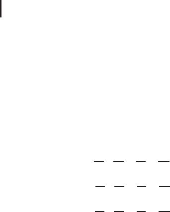
Fig. 4.30 (a) Applanation tonometry measurement proce-
dure. (b) Boundaries of the three-dimensional eye model.
Applanation tonometry is based on Goldmann’s assumption that the rigidity of the
human cornea does not vary much between individuals. Recently, however, it has
been shown that this assumption is wrong. Indeed, the rigidity of the human cornea
varies substantially between individuals due to natural variations of the thickness
of the cornea [212], and due to variations of the biomechanical properties (such as
Young’s modulus) of the corneal tissue [213, 214]. As a consequence of the variable
rigidity of the human cornea, the measurement values obtained by Goldmann
applanation tonometry can deviate substantially from the real IOP [214, 215].
To be able to correct applanation tonometry measurements for the effects of
corneal rigidity variations, a mathematical model is needed that is able to pre-
dict tonometry measurements depending on a given corneal geometry and given
biomechanical properties of the corneal tissue. With this objective, a finite-element
model has been developed based on the equations discussed in the last section
and on a three-dimensional model of the human eye [215, 216]. An ‘‘average’’
three-dimensional eye geometry based on the data in [213] was used in the simu-
lations (Figures 4.30b and 4.31). Note that as Figure 4.30a shows, the cornea sits
on top of the sclera, and both structures together form a thin, shell-like structure,
which is known as the corneo-scleral shell. Figure 4.30b shows the boundaries of the
eye model where the following boundary conditions are applied:
•
Boundary 1: Corneal area that is flattened by the tonometer
head. A ‘‘flatness condition’’ is imposed here, which can be
realized iteratively as described in [217]
•
Boundaries 2,3: Outer surface of the eye. Atmospheric
pressure is prescribed here.
•
Boundary 4: Here, the outer eye hemisphere is in contact
with the inner hemisphere. Since this is ‘‘far away’’ from the
cornea, a no displacement condition or u = 0 is assumed here.
308 4 Mechanistic Models II: PDEs
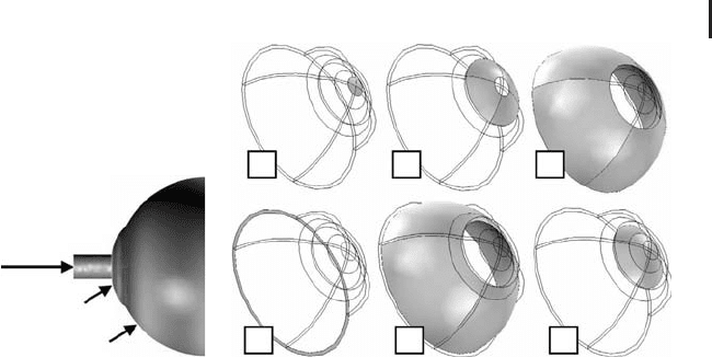
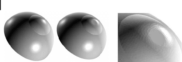
(a) (b) (c)
Fig. 4.31 Three-dimensional eye model: undeformed (a) and
deformed by the tonometer head (b and c).
•
Boundaries 5,6: Internal surface of the corneo-scleral shell.
The IOP acts on these surfaces, so the IOP is prescribed
there.
To simulate the deformation of the corneo-scleral shell based on these boundary
conditions and the equations described in the last section, an appropriate material
model for the stress–strain relation is needed. Typically, stress–strain relations of
biological tissues are nonlinear [218]. Unfortunately, the nonlinear stress–strain
behavior of the corneo-scleral shell has not yet been sufficiently characterized by
experimental data [214]. Hence, the simulation shown in Figure 4.31 is based
on a linear material model that uses Young’s moduli within the range that is
reported in the literature: a constant Young’s modulus of 0.1 MPa in the cornea
[213, 214], and 5.5 MPa in the sclera [213, 219]. Following [214], Poisson’s ratio
was set to a constant value of ν = 0.49 in the entire corneo-scleral shell. Note
that this simulation has been performed using the ‘‘structural mechanics module’’
of the commercial Comsol Multiphysics. You can do the same simulation using
Code_Aster based on CAELinux as described above (Comsol Multiphysics was used
here to test some nonlinear material models that are currently unavailable in
Code_Aster).
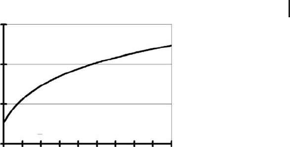
The simulations can be used to estimate the measurement error of Goldmann
applanation tonometry. Figure 4.32 shows the effect of scleral rigidity variations
on the simulated IOP reading. In this figure, a scleral rigidity corresponding to a
Young’s modulus of 5.5 MPa is assumed as a ‘‘reference rigidity’’. Then, the scleral
Young’s modulus is varied between 1 and 10 MPa, which is the (approximate)
range of scleral Young’s moduli reported in the literature [213, 219]. What the
figure shows is the percent deviation of the simulated IOP reading from the
IOP reading that is obtained in the reference situation. As the figure shows,
the IOP reading can deviate by as much as 7% based on the variations of the
scleral rigidity only. As expected, the effect of the corneal rigidity is even higher
and can amount to 25–30% within the range of rigidities that is reported in the
literature.
4.11 Other Mechanistic Modeling Approaches 309
5
0
−5
−10
11098765432
Scleral Young’s modulus (Mpa)
Deviation from reference (%)
Fig. 4.32 Effect of scleral rigidity variations on the simulated IOP reading.
4.11
Other Mechanistic Modeling Approaches
At this point, similar remarks apply as in the case of phenomenological modeling
(Section 2.7): Again, you should be aware of the fact that there is a great number of
mechanistic modeling approaches beyond those that are discussed in this chapter
and in chapter 3. We will confine ourselves here to a few examples, which are by
no means exhaustive, but which may demonstrate how mathematical structures
different from the ones discussed above may arise.
4.11.1
Difference Equations
Consider a host–parasite system, where parasites use host plants to deposit their
eggs. Let
•
N
t
:numberofhostspeciesinthetth breeding season
(t = 1, 2, 3, ...);
•
P
t
: number of parasite species in the tth breeding season.
Then it can be argued that [220]
N
t+1
= λe
−γ P
t
N
t
(4.153)
P
t+1
= cN
t
1 −e
−γ P
t
(4.154)
where e
−γ P
t
is the fraction of hosts not parasitized (the particular form of this term
is a result of probabilistic considerations as explained in [220]), c is the average
number of eggs laid by surviving parasites, and λ isthehostgrowthrate,giventhat
all adults die before their offspring can breed.

310 4 Mechanistic Models II: PDEs
This model is known as the Nicholson–Bailey model. Althoughwewillnotgo
into a detailed discussion of these equations here, it is easy to understand the
message in qualitative terms: Equation 4.153 says that the hosts grow proportional
to the existing number of hosts, that is, in an exponential fashion similar to the
description of yeast growth in Section 3.10.2. If there are many parasites, e
−γ P
t
will
be close to zero, and hence the host growth rate will also go to zero. In a similar
way, Equation 4.154 expresses the fact that the number of parasites will increase
with the number of surviving eggs, the number of host species, and the number of
parasite species in the previous breeding season.
Mathematically, Equations 4.153 and 4.154 are classified as difference equations,
recurrence relations,ordiscrete models [114, 220]. Models of this kind are characterized
by the fact that the model equations can be used to set up an iteration that yields
a sequence of states such as (N
1
, P
1
), (N
2
, P
2
), .... In the above example and many
other applications of this kind, the iteration number t = 1, 2, 3, ... corresponds
to time, that is, time is treated as a discrete variable. Note the difference to
the differential equation models above, in which time and other independent
variables were treated as continuous quantities. As the above example shows,
finite difference models provide a natural setting for problems in the field of
population dynamics, but they can also be used to model other inherently discrete
phenomena, e.g. in the field of economics, traffic, or transportation flows [220,
221]. Difference equations such as Equations 4.153 and 4.154 can be easily
implemented using Maxima or R as described above. The iterations can be
formulated similar to the book software program
HeatClos.r that was discussed
in Section 4.6.3.
4.11.2
Cellular Automata
The concept of cellular automata was developed by John von Neumann and
Stanislaw Ulam in the early 1950s, inspired by the analogies between the operation
of computers and the human brain [222, 223]. We begin with a definition of cellular
automata and then consider an illustrative example [224]:
Definition 4.11.1 (Cellular automaton) A cellular automaton consists of
•
a regular, discrete lattice of cells (which are also called nodes or
sites) with boundary conditions;
•
a finite – typically small – set of states that characterizes the
cells;
•
a finite set of cells that defines the interaction neighborhood of
each cell; and
•
rules that determine the evolution of the states of the cells in
discrete time steps t = 1, 2, 3, ....
4.11 Other Mechanistic Modeling Approaches 311
(
a
)(
b
)
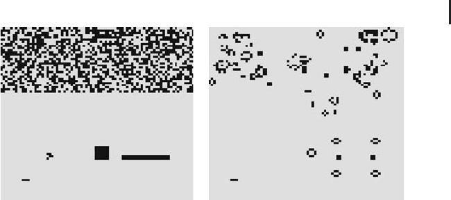
Fig. 4.33 Conway’s game of life computed using Conway.r:
(a) random initial state and (b) state after 100 iterations.
A simple example is the famous Conway’s Game of Life [225]. In this case, the
discrete lattice of cells is a square lattice comprising n × n cells, which we can think
of as representing individuals. These cells are characterized by two states called live
or dead. Figure 4.33 visualizes the states of each cell in such a square lattice using the
colors black (for life cells) and gray (for dead cells). The interaction neighborhood
of each cell comprises its eight immediate neighbors, and the interaction rules are
as follows:
•
Live cells with fewer than two live neighbors die (as if by
loneliness).
•
Live cells with more than three live neighbors die (as if by
overcrowding).
•
Live cells with two or three live neighbors survive.
•
Dead cells with exactly three live neighbors come to live
(almost as if by...).
Starting with some initial distribution of life and dead cells, these rules determine
iteratively the state of the ‘‘cell colony’’ at times t = 1, 2, 3, .... This algorithm has
been implemented by Petzoldt in [141] using R’s
simcol package. You may find
this example in the file
Conway.r in the book software. Figure 4.33a shows the
initial state of the cellular automaton generated by
Conway.r, and Figure 4.33b
shows the state that is attained after 100 iterations. Using
Conway.r on your own
computer, you will also be able to see the various intermediate states of the cellular
automaton on your computer screen. The example shows that a quite complex
behavior of a system may arise by the application of very simple rules.
Generally, cellular automata can be used to explain spatiotemporal patterns that
are caused by the interaction of cell-like units. Again, there is an abundant number
of applications in many fields. Cellular automata, for example, have been used
to explain surface patterns on seashells [227]. Seashells are covered with pigment
cells that excrete a pigment depending on the activity of the neighboring pigment
cells, which corresponds exactly to the way in which an abstract cellular automaton

312 4 Mechanistic Models II: PDEs
works. In [228], cellular automata have been used to explain the spreading of genes
conferring herbicide resistance in plant populations. Recently, it has been shown
that the gas exchange of plants can be explained based on cellular automata [229].
See [224] for many more biological applications and [230] for applications in other
fields such as the modeling of chemical reactions or of fluids.
4.11.3
Optimal Control Problems
In many practical applications of ODEs, one wants to control the process that is
expressed by the ODE in a way such that it behaves optimal in the sense that
it maximizes or minimizes some performance criterion. As an example, we may
think of the wine fermentation model that was discussed in Section 3.10.2. In
that case, it is important to control the temperature T(t) inside the fermenter in
an optimal way, for example, in a way such that the amount of residual sugar is
minimized.
Beyond a really abundant number of examples of this kind in the field of
technology (but also, e.g. in the field of economics, see [231]), there is also a
great number of applications pertaining to natural systems. Indeed, optimality is
important in nature as well as in technology – just think of Darwin’s theories of
evolution and the underlying idea of the ‘‘survival of the fittest’’. As an example, let
us consider the maintenance investment problem in plants stressed by air pollutants.
Generally, plants use the carbohydrates that are constantly produced in the process
of photosynthesis for two main purposes:
•
for maintenance processes: that is, to supply energy that is used
to repair damaged cell components and to resynthesize
degraded enzymes.
•
for growth: to build up new cells and plant structures.
In the presence of air pollutants, a decrease in the rate of photosynthesis
(measured e.g. as g CO
2
/g dry matter/day) is often observed. In many cases, this
is caused by the fact that the air pollutants destroy important enzymes such as the
RuBisCo enzyme [232]. This means that plants stressed by air pollutants need to
do more maintenance work, and hence they need more carbohydrates to supply
the necessary energy for maintenance. These carbohydrates are no longer available
for growth. Hence, the plant has to solve the following problem:
How much carbohydrates should be invested into maintenance and growth,
respectively?
In view of Darwin’s theory of evolution, this can be formulated as an optimization
problem as follows:
How much carbohydrates should be invested into maintenance and growth such
that the plant maximizes its reproductive success?

4.11 Other Mechanistic Modeling Approaches 313
Based on a very simple optimal control problem, it can be shown that real plants
indeed determine their carbohydrate investment into maintenance by solving a
problem of this kind [134, 135]. Let
•
N (g dry matter): ‘‘nonactive’’ overall biomass of the plant;
basically, a measure of the size of the plant
•
d (g dry matter/g dry matter): concentration of ‘‘degradable
biomass’’ within the plant; basically the concentration of
enzymes and other ‘‘degradable biomass’’ that is constantly
repaired and resynthesized in the plants maintenance
operations
The dynamical behavior of these two quantities can be described by the following
ODE system:
˙
N(t) = r(1 − u(t))φ(d(t))N(t) (4.155)
˙
d(t) = u(t)ρφ(d(t)) − σ d(t) − r(1 − u(t))φ(d(t))d(t) (4.156)
where t is time and the dot on the left-hand side of the equations denotes the time
derivative [134, 135]. In this ODE system, u(t) describes the amount of carbohydrates
that is invested into maintenance processes in percent, that is, u(t) ∈ [0, 1] (see [135]
for interpretations of the other parameters appearing in the equations). When the
plant solves the above optimization problem, it must ‘‘select’’ an optimal function
u(t), and since the plant, thus, virtually controls the performance of the system via
the selection of the optimal function u(t), the overall problem is called a control
problem or optimal control problem. Of course, a criterion must be specified as a part
of an optimal control problem that characterizes optimality. Above, it was said that
the plant decides about its maintenance investment in a way that maximizes its
reproductive success. In the framework of the above simple plant model, Equations
4.155 and 4.156, this can be expressed as
N(T) → max (4.157)
if the problem is solved in the time interval [0, T] ⊂ R. According to Equation
4.157, the plant is required to choose the maintenance investment u(t)inaway
that maximizes its nonactive biomass, that is, in a way that maximizes its size
(which is the best approximation of reproductive success maximization within this
model). In [135], this problem is solved in closed form using a technique called
Pontryagin’s principle. See [33, 233] for this and other closed form and numerical
solution techniques. These techniques apply to general systems of ODEs of the
form
y
(t) = F(t, y(t), u(t)) (4.158)
y(0) = y
0
(4.159)

314 4 Mechanistic Models II: PDEs
where t ∈ [0, T], y(t) = (y
1
(t), y
2
(t), ..., y
n
(t)) is the vector of state variables and u(t) =
(u
1
(t), u
2
(t), ..., u
m
(t)) is a vector of (time-dependent) control variables. Usually,
optimality is expressed in terms of a cost functional that is to be minimized:
φ(y(T)) +
T
0
L(y(t), u(t), t) dt → min (4.161)
which would give φ(N(T), d(T)) =−N(T) in the maintenance investment problem
discussed above.
4.11.4
Differential-algebraic Problems
In Section 3.5.7, a system of first-order ODEs was defined to be an equation of the
form:
y
(t) = F(t, y(t)) (4.162)
In the applications, this equation may also appear in the more general form
F(t, y(t), y
(t)) = 0 (4.163)
If Equation 4.163 cannot be brought into the form of Equation 4.162, it is
called an implicit ODE, while Equation 4.162 is an explicit ODE. Ascanbe
expected, more sophisticated solution procedures are needed to solve implicit
ODEs. Many equations of the form (4.163) can be described as a combination
of an ODE with algebraic conditions. Equations of this type are also known as
differential-algebraic equations (DAEs) [107, 112, 234, 235]. They may appear in
a number of different fields, such as mechanical multibody systems (includes
robotics applications), electrical circuit simulation, chemical engineering, control
theory, and fluid dynamics.
4.11.5
Inverse Problems
Remember Problem 2 from Section 4.1.3, which asked for the three-dimensional
temperature distribution within a cube. This problem was solved in Section 4.9
based on the stationary heat equation:
∇
K(x) ·∇T(x, t)
= 0 (4.164)
As a result, the three-dimensional temperature distribution T(x) within the cube
was obtained. As was already explained in Section 1.7.3, a problem of this kind is
called a direct problem, since a mathematical model (the heat equation) is used here
to obtain the output of the system ‘‘cube’’ (temperature in this case) based on a
given input (the boundary conditions imposed in Problem 2) and based on given