Velten K. Mathematical Modeling and Simulation: Introduction for Scientists and Engineers

Подождите немного. Документ загружается.

4.6 The Finite Difference Method 265

Section 4.5. Principally, problems of this kind can be solved as matrix equations

using the standard methods of linear algebra such as Gaussian elimination and

LU decomposition techniques [159]. This kind of solution methods are called direct

solution methods since they solve the general matrix problem Ax = b in a single

step, basically by inverting the matrix A. Direct methods, however, are usually

expensive in terms of computer memory since you need to keep the matrix (at least

the nonzero elements) in the memory, and also in terms of their computational

requirements, that is, in terms of the number of arithmetical operations needed

until the solution is obtained [160]. This is a problem even though the matrices

arising in the numerical treatment of PDEs are usually sparse matrices in the sense

that most matrix entries are zero, which reduces the memory requirements.

Thus, linear equations derived from PDEs are usually solved based on another

class of methods called iterative methods. These methods start with an initial guess

for the unknowns, which is then successively improved until a sufﬁciently precise

approximation of the solution of the PDE is achieved. In the above example, we

could start with an initial guess U

(0)

i,j

(i, j = 0, ..., N)andthenuseEquation4.99to

compute U

(1)

i,j

, U

(2)

i,j

, ...from

(k+1)

i,j



(k)

i+1,j

+ U

(k)

i−1,j

+ U

(k)

i,j+1

+ U

(k)

i,j−1



+ πρ

i,j



(4.100)

This particular iterative method is called the Jacobi method, but there are more

effective methods such as the Gauss–Seidel method and relaxation methods,which

are discussed in [111, 160]. In [111] you may ﬁnd an example application of Equation

4.99, along with a program solving this equation using a relaxation method.

Note 4.6.1 (Nested iterations) The numerical solution of nonlinear PDEs may

involve several nested iterations (which often can be observed in the output of

PDE solving software): for example, outer iterations resolving the time scale (for

instationary equations) and/or the nonlinearity (Section 4.3.1.3), and an inner

iteration solving the resulting system of linear equations.

4.6.8

Billions of Unknowns

As was just mentioned, iterative methods are used mainly due to the large size of

the linear equation systems derived from PDEs, which may increase the memory

and computation time requirements of direct methods beyond all limits. Referring

to the FD approach just discussed, it can be demonstrated why the linear equation

systems derived from PDEs can be so large. Assume we want to use the FD method

to compute some unknown quantity U inthecube[0,1]

. Let us assume that we

use the same spatial step  = 1/N (N ∈ N) in all three space directions. Then, an

application of the FD method similar to above would generate a linear equation

266 4 Mechanistic Models II: PDEs

system with about N

unknowns U

i,j,k

(the real number of unknowns may be

slightly different due to the application of the appropriate boundary conditions.)

The value of N will depend on your application. N = 10 may be sufﬁcient in some

cases, which would give about N

= 1000 unknowns. If, however, your application

requires a very ﬁne resolution, you might need N = 100 and then come up with an

overall number of unknowns in the order of millions.

Now you should note that this example refers to the computation of only one state

variable U. Many applications require the solution of systems of PDEs involving

the computation of several state variables on your computational grid, for example,

the pressure and several velocity components in CFD applications. In the N = 1000

case, you would get a billion unknowns for each of your state variables. Then, you

may want to observe the development of your state variables in time, that is,

you may want to solve your problem as an instationary problem, which means

you have to solve problems involving billions of unknowns in every single time

step of your numerical algorithm. In applications of the FE method (Section 4.7),

your geometry may involve tiny structures that need to be resolved by a very ﬁne

computational grid, and again every point of that ﬁne grid will increase the number

of the unknowns. In this way, your PDE application may easily generate far more

than a billion unknowns, and hence it is not surprising that the solution of PDEs

can be very expensive in terms of memory requirements and computation time.

Note 4.6.2 (Need for computational efﬁciency) Computational efﬁciency is an

important issue in the numerical treatment of PDEs. It involves a proper analysis

of the dimensionality and symmetry of the problem (Section 4.3.3) as well as the

use of fast and efﬁcient iterative methods to solve the equations.

Note that N = 100 would generate only about 10 000 unknowns (instead of a

million) if you can solve the problem in 2D (instead of 3D), or about 500 000

unknowns would sufﬁce if you can do your computation in half of the original

domain due to symmetry considerations.

4.7

The Finite-Element Method

As was discussed in Section 4.5, a main disadvantage of the FD method is its

lack of geometrical ﬂexibility. It always needs regular computational grids to be

mapped onto the computational domain, which restricts the complexity of the

geometries that can be treated. The ﬁnite-element method (FE method), on the

other hand, is particularly well suited for complex geometries. It uses grids made

up of simple geometrical forms such as triangles in 2D or tetrahedra in 3D. These

simple geometrical forms are called ﬁnite elements, and by putting together a great

number of these ﬁnite elements virtually any imaginable geometrical object can be

4.7 The Finite-Element Method 267

(a) (b)

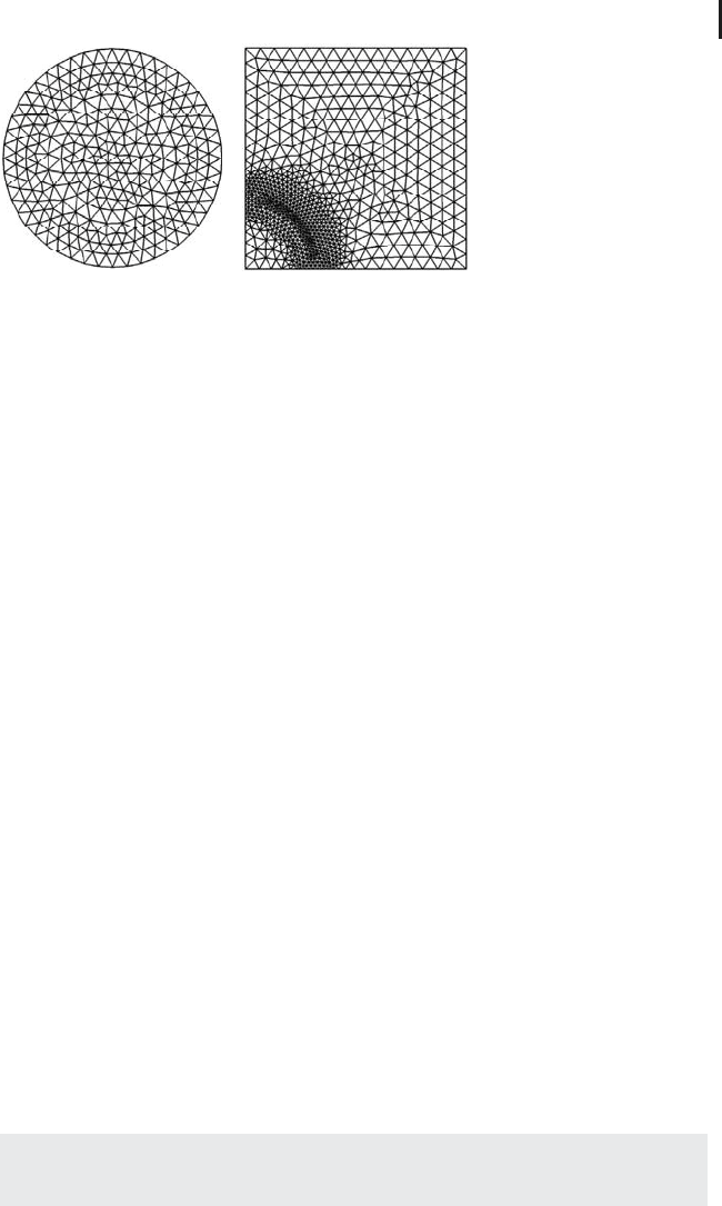
Fig. 4.7 (a) Example triangulation of a circle. (b) Example of a locally reﬁned mesh.

constructed. As an example, Figure 4.7a shows the construction of a circular domain

using triangles as ﬁnite elements. A construction as in Figure 4.7a is called a mesh

or grid, and the generation of a mesh covering the geometry is an important step of

the ﬁnite-element method (see the discussion of mesh generation using software

in Section 4.8). If a 2D grid is constructed using triangles similar to Figure 4.7a,

the resulting mesh is also called a triangulation of the original geometry.

Note that the geometry shown in Figure 4.7a cannot be covered by the structured

grids that are used in the FD method (Section 4.6). The grid shown in Figure 4.7a

is called an unstructured grid, since the crossing points of the grid – which are also

called the knots of the grid – do not have any kind of regular structure (e.g. in

contrast to the FD grids, they do not imply any natural ordering of these crossing

points). Similar to the FD method, the crossing points of an FE mesh are the points

where the numerical algorithm produces an approximation of the state variables

(more precisely, weights of basis functions are determined at the crossing points,

see below). Depending on your application, you might need a higher or lower

resolution of the numerical solution – and hence a higher or lower density of those

crossing points – in different regions of the computational domain. This can be

realized fairly easily using unstructured FE meshes. Figure 4.7b shows an example

where a much ﬁner grid is used in a circular strip. Such meshes are called locally

reﬁned meshes. Locally reﬁned meshes can not only be used to achieve a desired

resolution of the numerical solution but may also help to circumvent inherent

problems with the numerical algorithms [161–163].

4.7.1

Weak Formulation of PDEs

The difference between the computational approaches of the FD and FE methods

can be phrased as follows:

Note 4.7.1 TheFDmethodapproximatestheequationandtheFEmethod

approximates the solution.

268 4 Mechanistic Models II: PDEs

To make this precise, consider the Poisson equation in 2D (Section 4.6.6):

∂

U(x , y)

∂x

∂

U(x , y)

∂y

= f (x, y) (4.101)

where (x, y) ∈  ⊂ R

and f is some real function on . Now following the idea

of the FD approach and using the central difference approximation described in

Section 4.6.1, this equation turns into the following difference equation:

U(x + x, y) +U(x − x, y) −2U(x, y)

x

U(x , y + y) +U(x, y − y) − 2U(x, y)

y

= f (x, y)

(4.102)

Equation 4.102 approximates Equation 4.101, and in this sense it is valid to

say that ‘‘the FD method approximates the equation’’. Now to understand what

it means that the ‘‘FE method approximates the solution’’, let us consider a 1D

version of Equation 4.101:



(x) = f (x) x ∈ (0, 1) (4.103)

u(0) = u(1) = 0 (4.104)

Of course, this is now an ODE, but this problem is, nevertheless, very well suited

to explain the idea of the FE method in simple terms. Let v be a smooth function

which satisﬁes v(0) = v (1) = 0. Here, ‘‘smoothness’’ means that v is assumed to be

inﬁnitely often differentiable with compact support, which is usually denoted as

v ∈ C

∞

(0, 1), see [138] (we do not need to go into more details here since we are

not going to develop a theory of PDEs). Equation 4.103 implies





(x)v(x) dx =



f (x)v(x) dx (4.105)

Using v(0) = v(1) = 0, an integration by parts of the left-hand side gives

−





(x)v



(x) dx =



f (x)v(x) dx (4.106)

Let H

(0, 1) be a suitable set of real functions deﬁned on (0, 1). H

(0, 1) is a

so-called Sobolev space, which is an important concept in the theory of PDEs (see

the precise deﬁnitions in [138]). Deﬁning

φ(u, v) =





(x)v



(x) dx (4.107)

for u, v ∈ H

(0, 1), it can be shown that the following problem is uniquely solv-

able [80]:

Find u ∈ H

(0, 1) such that

∀v ∈ H

(0, 1) : −φ(u, v) =



f (x)v(x) dx

(4.108)

4.7 The Finite-Element Method 269

Problem (4.108) is called the variational formulation or weak formulation of

Equations 4.103 and 4.104. Here, the term weak is motivated by the fact that some

of the solutions of problem (4.108) may not solve Equations 4.103 and 4.104 since

they do not have a second derivative in the usual sense, which is needed in Equation

4.103. Instead, solutions of problem (4.108) are said to be weakly differentiable,and

these solutions themselves are called weak solutions of the PDE in its original

formulation, that is, of Equations 4.103 and 4.104. Although we conﬁne ourselves

to a discussion of Equations 4.103 and 4.104 here, you should note that similar

weak formulations can be derived for linear second-order PDEs in general, and

these weak formulations can then also be approximated in a similar way using

ﬁnite elements as will be explained below [138].

4.7.2

Approximation of the Weak Formulation

The idea of the ﬁnite-element method is to replace the inﬁnite-dimensional space

(0, 1) by a ﬁnite-dimensional subspace V ⊂ H

(0, 1), which turns Equation 4.108

into the following problem:

Find u ∈ V such that

∀v ∈ V : −φ(u, v) =



f (x)v(x) dx

(4.109)

Remember from your linear algebra courses that the dimension of a vector

space V is n ∈ N if there are linear independent basis vectors v

, ..., v

∈ V that

can be used to express any w ∈ V as a linear combination w = a

+···+a

, ..., a

∈ R ). For the space H

(0, 1) used in problem (4.108), no such basis can

be found which means that this is an inﬁnite-dimensional space [138]. Such a space

is unsuitable for a numerical algorithm that can perform only a ﬁnite number of

steps, and this is why problem (4.108) is replaced by problem (4.109) based on the

ﬁnite-dimensional subspace V.Ifv

, ..., v

is a set of basis functions of V,any

function u ∈ V canbewrittenas

u =



j=1

(4.110)

where u

, ..., u

∈ R . Problem (4.109) can now be written as

Find u

, ..., u

∈ R such that for i = 1, ..., n

−



j=1

φ(v

, v

) ·u



(x)f (x) dx

(4.111)

Using the deﬁnitions

A = (φ(v

, v

))

i=1...n,j=1...n

(4.112)

u = (u

)

j=1...n

(4.113)

f =





(x)f (x) dx



i=1...n

(4.114)

270 4 Mechanistic Models II: PDEs

problem (4.111) can be written in matrix form as follows:

Find u ∈ R

such that

A · u = f

(4.115)

The FE method thus transforms the original PDE Equations 4.103 and 4.104 into

a system of linear equations, as was the case with the FD method discussed above.

Remember that it was said above that the FD method approximates the equation

expressing the PDE, while the FE method approximates the solution of the PDE

(Note 4.7.1). This can now be made precise in terms of the last equations. Note

that the derivation of Equation 4.115 did not use any discrete approximations of

derivatives, which would lead to an approximation of the equation expressing the

PDE similar to the FD method. Instead, Equation 4.110 was used to approximate the

solution of the PDE – which lies in the inﬁnite-dimensional Sobolev space H

(0, 1)

as explained above – in terms of the ﬁnite-dimensional subspace V ⊂ H

(0, 1).

4.7.3

Appropriate Choice of the Basis Functions

To simplify the solution of Equation 4.115, the basis v

, ..., v

of V is chosen in

a way that turns the matrix A into a sparse matrix, that is, into a matrix with most

of its entries being zero. Based on a decomposition of [0, 1] into 0 = x

< x

···< x

n+1

= 1, one can, for example, use the piecewise linear functions

(x) =

⎧

⎪

⎨

⎪

⎩

x − x

k−1

− x

k−1

if x ∈

[

k−1

, x

]

k+1

− x

k+1

− x

if x ∈

[

, x

k+1

]

0otherwise

(4.116)

Then, the functions v

for k = 1, ..., n span up an n-dimensional vector space

V thatcanbeusedasanapproximationofH

(0, 1) as discussed above. More

precisely, these functions span up the vector space of all functions being piecewise

linear on the subintervals [x

k−1

, x

](k = 1, ..., n + 1). In terms of our above

discussion, 0 = x

< x

···< x

n+1

= 1 deﬁnes a decomposition of [0, 1] into

ﬁnite elements where the subintervals [x

k−1

, x

] are the ﬁnite elements, and the

mesh (or grid) consists of the points x

, ..., x

n+1

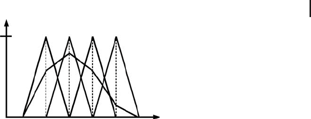
Figure 4.8 shows an example for n = 4. The ﬁgure shows four ‘‘hat functions’’

centered at x

, x

corresponding to the basis functions v

, v

,anda

function being piecewise linear on the subintervals [x

k−1

, x

](k = 1, ...,5), which

is some linear combination of the v

such as

u(x) =



k=1

(x) (4.117)

4.7 The Finite-Element Method 271

= 0

= 1

Fig. 4.8 Example one-dimensional ‘‘hat’’ basis functions, and

a piecewise linear function generated by a linear combina-

tion of these basis functions.

where a

, a

∈ R .Sincev

is nonzero only on the interval [x

k−1

, x

k+1

], the

entries of the matrix A in Equation 4.115

φ(v

, v

) =





(x)v



(x) dx (4.118)

are zero whenever |i − j| > 1, which means that these basis functions, indeed,

generate a sparse matrix A as discussed above. Obviously, the sparsity of A is a

consequence of the fact that the basis functions v

are zero almost everywhere.

Since the set of points where a function gives nonzero values is called the support

of that function, we can say that a basic trick of the FE method is to use basis

functions having a small support.

4.7.4

Generalization to Multidimensions

The same procedure can be used for higher-dimensional PDE problems. For

example, to solve the Poisson equation (4.101), the ﬁrst step would be to ﬁnd an

appropriate weak formulation of Equation 4.101 similar to Equation 4.108. This weak

formulation would involve an appropriate Sobolev Space of functions, which would

then again be approximated by some ﬁnite-dimensional vector space V. Asabasis

of V, piecewise linear functions could be used as before (although there are many

alternatives [138]). A decomposition of [0, 1] into 0 = x

< x

···< x

n+1

= 1

was used above to deﬁne appropriate piecewise linear functions. In 2D, the

corresponding step is a decomposition of the two-dimensional domain into ﬁnite

elements, similar to the decomposition of a circular domain into triangles in

Figure 4.7a. In analogy with the above discussion, one would then use piecewise

linear basis functions v

, which yield 1 on one particular crossing point of the

ﬁnite-element grid and 0 on all other crossing points. Using linear combinations of

272 4 Mechanistic Models II: PDEs

these basis functions, arbitrary piecewise linear functions can then be generated.

In 3D, the same procedure can be used, for example, based on a decomposition of

the computational domain in tetrahedra (Section 4.9.2 and Figure 4.17).

The FE method as described above is an example of a more general approach

called the Galerkin method [161, 162], which applies also, for example, to the

boundary element method for solving integral equations [164, 165] or to Krylov

subspace methods for the iterative solution of linear equation systems [160].

4.7.5

Summary of the Main Steps

The general procedure of the FE method can be summarized as follows:

Main steps of the FE method

1. Geometry deﬁnition: deﬁnition of the geometry of the domain in

which the PDE is to be solved.

2. Mesh generation: decomposition of the geometry into geometric

primitives called ﬁnite elements (e.g. intervals in 1D, triangles in

2D, and tetrahedra in 3D).

3. Weak problem formulation: formulationofthePDEinweakform.

Finite-dimensional approximation of the weak problem using

the mesh.

4. Solution: solution of a linear equation system derived from the

weak problem or of an iterated sequence of linear equation

systems in the case of nonlinear and/or instationary PDEs (Note

4.6.1).

5. Postprocessing: generation of plots, output ﬁles, and so on.

The geometry deﬁnition step corresponds to the deﬁnition of the interval [0, 1] in

the above discussion of Equations 4.103 and 4.104. If we want to solve, for example,

the two-dimensional Poisson equation (4.101) in a circular domain, this step would

involve the deﬁnition of that circular domain. Although these examples are simple,

geometry deﬁnition can be quite a complex task in general. For example, if we want

to use the PDEs of CFD to study the air ﬂow within the engine of a tractor, the

complex geometry of that engine’s surface area needs to be deﬁned. In practice, this

is done using appropriate CAD software tools. FE software (such as Salome-Meca,

Section 4.8) usually offers at least some simple CAD tools for geometry construction

as well as options for the import of ﬁles generated by external CAD software.

The mesh generation step involves the decomposition of the geometry into ﬁnite

elements as discussed above. Although triangles (in 2D) and tetrahedra (in 3D) are

used in most practical applications, all kinds of geometrical primitives can be used

here in principle. For example, some applications use rectangles or curvilinear

shapes in 2D or hexahedra, prisms, or pyramids in 3D. Of course, mesh generation

4.7 The Finite-Element Method 273

is an integral part of any FE software. Efﬁcient algorithms for this task have been

developed. An important issue is the mesh quality generated by these algorithms,

that is, the compatibility of the meshes with the numerical solution procedures.

For example, too small angles in the triangles of a FE mesh can obstruct the

numerical solution procedures, and this can be avoided, for example, by the use

of Delaunay triangulations [166]. Another important aspect of mesh generation is

mesh reﬁnement. As was discussed above, one might want to use locally reﬁned

meshes such as the one shown in Figure 4.7b to achieve the desired resolution

of the numerical solution or to avoid problems with the numerical algorithms.

FE software such as Salome-Meca offers a number of options to deﬁne locally

reﬁned meshes as required (Section 4.9.2). The mesh generation step may also be

coupled with the solution of the FE problem in various ways. For example, some

applications require ‘‘moving meshes’’, such as coupled ﬂuid–structure problems

where a ﬂowing ﬂuid interacts with a deforming solid structure [167]. Some

algorithms use adaptive mesh reﬁnement strategies where the mesh is automatically

reﬁned or coarsened depending on a posteriori error estimates computed from the

numerical solution [139].

The weak problem formulation step is the most technical issue in the above

scheme. This step involves, for example, the selection of basis functions of the

ﬁnite-dimensional subspace V in which the FE method is looking for the solution.

In the above discussion, we used piecewise linear basis functions, but all kinds of

other basis functions such as piecewise quadratic or general piecewise polynomial

basis functions can also be used [166]. Note that some authors use the term ﬁnite

element as a name for the basis functions, rather than for the geometrical primitives

of the mesh. This means that if you read about ‘‘quadratic elements’’, the FE method

is used with second-order polynomials as basis functions. If the PDE is nonlinear,

the weak problem formulation must be coupled with appropriate linearization

strategies [139]. Modern FE software such as Salome-Meca (Section 4.8) can be used

without knowing too much about the details of the weak problem formulation step.

Typically, the software will use reasonable standard settings depending on the PDE

type speciﬁed by the user, and as a beginner in the FE method it is usually a good

idea to leave these standard settings unchanged.

The solution step of the FE method basically involves the solution of linear

equation systems involving sparse matrices as discussed above. As was mentioned

in Section 4.6.7, large sparse linear equation systems are most efﬁciently solved

using appropriate iterative methods. In the case of instationary PDEs, the FE

method can be combined with a treatment of the time derivative similar as was

done above for the heat equation (Section 4.6). Basically, this means that a sequence

of linear equation systems must be solved as we move along the time axis [166]. In

the case of nonlinear PDEs, the FE method must be combined with linearization

methods such as Newton’s method [139], which again leads to the solution of an

iterated sequence of linear equation systems. Again, all this as well as the ﬁnal

postprocessing step of the FE method is supported by modern FE software such as

Salome-Meca (Section 4.8).

274 4 Mechanistic Models II: PDEs

Note 4.7.2 (Comparison of the FD and FE methods) The FD method is relatively

easy to implement (Section 4.6), but is restricted to simple geometries. The FE

method can treat complex geometries, but its implementation is a tedious task

and so it is usually efﬁcient to use existing software tools such as Salome-Meca.

4.8

Finite-element Software

As was mentioned above, the software implementation of the FE method is a

demanding task, and this is why most people do not write their own FE programs.

A great number of both open-source and commercial FE software packages are

available, see Table 4.1 for a list of examples which is by no means exhaustive.

Generally speaking, there is a relatively broad gap between open-source and

commercial FE software. It is relatively easy to do your everyday ofﬁce work, for

example, using the open-source OpenOfﬁce software suite instead of the commercial

Microsoft Ofﬁce package, or to perform a statistical analysis using the open-source

R package instead of commercial products such as SPSS, but it is much less easy

to work with open-source FE software if you are used to commercial products

such as Fluent or Comsol Multiphysics. Given a particular FE problem, it is highly

likely that you will ﬁnd open-source software that can solve your problem, but

you will need time to understand that software before you can use it. Having

solved that particular problem, your next problem may be beyond the scope of that

software, so you may have to ﬁnd and understand another suitable open-source

FE package. The advantages of commercial FE software can be summarized as

follows:

•

Range of application: commercial FE software usually

provides a great number of models that can be used.

•

User-friendliness: commercial FE software usually provides

sophisticated graphical user interfaces, a full integration of

all steps of the FE analysis from the geometry deﬁnition to

the postprocessing step (Section 4.7.5), a user friendly

workﬂow involving, for example, the extraction of

parameters from material libraries, and so on.

•

Quality: commercial FE software usually has been

thoroughly tested.

•

Maintenance and support: commercial FE software usually

provides a continuous maintenance and support.

Of course, these points describe the general advantages of commercial software

not only in the ﬁeld of ﬁnite-element analysis. All these have particular relevance

here due to the complexity of this kind of analysis: an enormous amount of

resources is needed to set up general FE software packages such as Fluent or

Comsol Multiphysics.