Versteeg H., Malalasekra W. An Introduction to Computational Fluid Dynamics: The Finite Volume Method
Подождите немного. Документ загружается.


7.5 EXAMPLES 217
Solution with the back-substitution formula (7.6a),
φ
j
= A
j
φ
j+1
+ C ′
j
, gives
φ
5
= 0 + 21.30
= 21.30
φ
4
= 0.3816 × 21.30 + 14.4735
= 22.60
φ
3
= 0.3793 × 22.60 + 17.9308
= 26.50
φ
2
= 0.3636 × 26.50 + 27.2727
= 36.91
φ
1
= 0.25 × 36.91 + 55
= 64.23
Nodes 1 and 5 are boundary nodes so we set
β
1
= 0 and
α
5
= 0. The
φ
at the
boundaries is not used; the boundary conditions enter into the calculation
through the source terms C
j
.
To show the results most clearly the values of
α
,
β
, D and C are given
for each node in Table 7.1, and A
j
and C ′
j
, calculated using the recurrence
formulae (7.6b) and (7.6c), are given in Table 7.2.
Table 7.1
Node
ββ
j
D
j
αα
j
C
j
A
j
C ′
j
1 0 20 5 1100 0.25 55
2 5 15 5 100 0.3636 27.2727
3 5 15 5 100 0.3793 17.9308
4 5 15 5 100 0.3816 14.4735
5 5 10 0 100 0.00 21.3009
Table 7.2 Specimen calculation
A
j
= C ′
j
=
A
1
==0.25 C ′
1
==55
A
2
==0.3636 C ′
2
==27.2727
A
3
==0.3793 C ′
3
==17.9308
A
4
==0.3816 C ′
4
==14.4735
A
5
= 0 C ′
5
==21.3009
5 × 14.4735 + 100
(10 − 5 × 0.3816)
5 × 17.9308 + 100
(15 − 5 × 0.3793)
5
(15 − 5 × 0.3793)
5 × 27.2727 + 100
(15 − 5 × 0.3636)
5
(15 − 5 × 0.3636)
5 × 55 + 100
(15 − 5 × 0.25)
5
(15 − 5 × 0.25)
0 + 1100
(20 − 0)
5
(20 − 0)
β
j
C ′
j−1
+ C
j
D
j
−
β
j
A
j−1
α
j
D
j
−
β
j
A
j−1
ANIN_C07.qxd 29/12/2006 04:48PM Page 217
The two-dimensional steady state heat transfer in the plate is governed by
k + k = 0 (7.11)
This can be written in discretised form as
a
P
T
P
= a
W
T
W
+ a
E
T
E
+ a
S
T
S
+ a
N
T
N
(7.12a)
where
a
W
= A
w
a
E
= A
e
a
S
= A
s
a
N
= A
n
(7.12b)
a
P
= a
W
+ a
E
+ a
S
+ a
N
(7.12c)
In this case, the values of all neighbour coefficients are equal:
a
W
= a
E
= a
N
= a
S
=×(0.1 × 0.01) = 10
At interior points 6 and 7
a
P
= a
W
+ a
E
+ a
S
+ a
N
= 40
1000
0.1
k
∆y
k
∆y
k
∆x
k
∆x
D
E
F
∂
T
∂
y
A
B
C
∂
∂
y
D
E
F
∂
T
∂
x
A
B
C
∂
∂
x
218 CHAPTER 7 SOLUTION OF DISCRETISED EQUATIONS
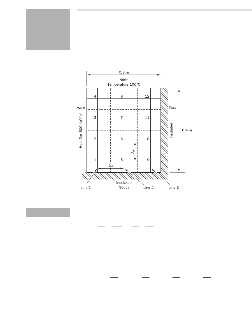
In Figure 7.4 a two-dimensional plate of thickness 1 cm is shown. The
thermal conductivity of the plate material is k = 1000 W/m.K. The west
boundary receives a steady heat flux of 500 kW/m
2
and the south and east
boundaries are insulated. If the north boundary is maintained at a tem-
perature of 100°C, use a uniform grid with ∆x =∆y = 0.1 m to calculate the
steady state temperature distribution at nodes 1, 2, 3, 4, . . . etc.
Figure 7.4 Boundary conditions
for the two-dimensional heat
transfer problem described in
Example 7.2
Solution
Example 7.2
A two-
dimensional
line-by-line
application of
the TDMA
ANIN_C07.qxd 29/12/2006 04:48PM Page 218

7.5 EXAMPLES 219
so the discretised equation at point 6 is
40T
6
= 10T
2
+ 10T
10
+ 10T
5
+ 10T
7
All nodes except 6 and 7 are adjacent to boundaries.
At a boundary node the discretised equation takes the form
a
P
T
P
= a
W
T
W
+ a
E
T
E
+ a
S
T
S
+ a
N
T
N
+ S
u
a
P
= a
W
+ a
E
+ a
S
+ a
N
− S
p
The boundary conditions are incorporated into the discretised equations
by setting the relevant coefficient to zero and by the inclusion of source
terms through S
u
and S
p
. Otherwise, the procedure is the same as in the
one-dimensional Example 7.1. We demonstrate the approach by forming the
discretised equations for boundary nodes 1 and 4.
At node 1
West is a constant flux boundary; let b
W
be the contribution to the source
term from the west:
a
W
= 0
b
W
= q
w
. A
w
= 500 × 10
3
× (0.1 × 0.01) = 500
South is an insulated boundary; no flux enters the control volume through
the south boundary:
a
S
= 0
b
S
= 0
Total source
S
u
= b
W
+ b
S
= 500
S
p
= 0
The discretised equation at node 1 is
20T
1
= 10T
2
+ 10T
5
+ 500
At node 4
West is a constant flux boundary
a
W
= 0
b
W
= 500 × 10
3
× (0.1 × 0.01) = 500
North is a constant temperature boundary
a
N
= 0
b
N
= A
n
× 100 = 2000
S
P
N
=− A
n
=−20
Total source
S
u
= b
W
+ b
N
= 500 + 2000 = 2500
S
p
=−20
2k
∆y
2k
∆y
ANIN_C07.qxd 29/12/2006 04:48PM Page 219

Let us apply the TDMA along north–south lines, sweeping from west to
east. The discretisation equation is given by
−a
S
T
S
+ a
P
T
P
− a
N
T
N
= a
W
T
W
+ a
E
T
E
+ b (7.13)
For convenience the line in Figure 7.4 containing points 1 to 4 is referred to
as line 1, the one containing points 5 to 8 as line 2, and the one with points 9
to 12 as line 3. All west coefficients are zero at points 1, 2, 3 and 4: hence the
values to the west of line 1 do not enter into the calculation. East values
(points 5, 6, 7 and 8) are required for the evaluation of C. They are unknown
at this stage and are assumed to be zero as an initial guess. The values of
α
j
,
β
j
, D
j
and C
j
can be calculated using equations (7.2) and (7.13). Now we have
α
j
= a
N
,
β
j
= a
S
, D
j
= a
P
and C
j
= a
W
T
W
+ a
E
T
E
+ S
u
. The values of
α
j
,
β
j
,
D
j
and C
j
and A
j
and C ′
j
for line 1 are summarised in Table 7.4 and the
calculations for A
j
and C ′
j
in Table 7.5.
220 CHAPTER 7 SOLUTION OF DISCRETISED EQUATIONS
Table 7.4
Node
ββ
j
D
j
αα
j
C
j
A
j
C ′
j
1 0 20 10 500 0.5 25
2 10 30 10 500 0.4 30
3 10 30 10 500 0.385 30.769
4 10 40 0 2500 0 77.667
Now we have
a
p
= a
S
+ a
E
− S
P
= 10 + 10 + 20 = 40
S
u
= 2500
The discretised equation at node 4 is
40T
4
= 10T
3
+ 10T
8
+ 2500
The coefficients and the source term of the discretisation equation for all
points are summarised in Table 7.3.
Table 7.3
Node a
N
a
S
a
W
a
E
a
P
S
u
1 10 0 0 10 20 500
2 10 10 0 10 30 500
3 10 10 0 10 30 500
4 0 10 0 10 40 2500
5 10 0 10 10 30 0
6 101010 1040 0
7 101010 1040 0
8 0 10 10 10 50 2000
910010020 0
10 10 10 10 0 30 0
11 10 10 10 0 30 0
12 0 10 10 0 40 2000
ANIN_C07.qxd 29/12/2006 04:48PM Page 220

7.5 EXAMPLES 221
The TDMA solution for line 2 is T
5
= 27.38, T
6
= 30.03, T
7
= 38.47 and
T
8
= 63.23. We can now proceed to the third line containing points 9, 10, 11
and 12. The values of
α
j
,
β
j
, D
j
and C
j
are summarised in Table 7.7.
Solution by back-substitution gives
T
4
= 0 + 77.667
= 77.67
T
3
= 0.385 × 77.667 + 30.769
= 60.67
T
2
= 0.4 × 60.67 + 30
= 54.27
T
1
= 0.5 × 54.268 + 25
= 52.13
The TDMA calculation procedure for line 2 is similar to line 1. Here the
values to the west are known from the calculations given above and the
values to the east are assumed to be zero. We leave the detailed calculations
as an exercise for the reader. The values of
α
j
,
β
j
, D
j
and C
j
for points 5, 6, 7
and 8 are summarised in Table 7.6.
Table 7.5
A
j
= C ′
j
=
A
1
==0.5 C ′
1
==25
A
2
==0.4 C ′
2
==30
A
3
==0.385 C ′
3
==30.769
A
4
= 0 C ′
4
==77.667
10 × 30.769 + 2500
(40 − 10 × 0.385)
10 × 30 + 500
(30 − 10 × 0.4)
10
(30 − 10 × 0.4)
10 × 25 + 500
(30 − 10 × 0.5)
10
(30 − 10 × 0.5)
0 + 500
(20 − 0)
10
(20 − 0)
β
j
C ′
j−1
+ C
j
D
j
−
β
j
A
j−1
α
j
D
j
−
β
j
A
j−1
Table 7.6
Node
ββ
j
D
j
αα
j
C
j
5 0 30 10 521.3
6 10 40 10 542.6
7 10 40 10 606.5
8 10 50 0 2776.7
ANIN_C07.qxd 29/12/2006 04:48PM Page 221

7.5.1 Closing remarks
We have discussed the solution of systems of equations with the TDMA.
This algorithm is highly economical for tri-diagonal systems. It consists of a
forward elimination and a back-substitution stage:
• Forward elimination
– arrange system of equations in the form of (7.2):
−
β
j
φ
j−1
+ D
j
φ
j
−
α
j
φ
j+1
= C
j
– calculate coefficients
α
j
,
β
j
, D
j
and C
j
– starting at j = 2 calculate A
j
and C ′
j
using (7.6b–c):
A
j
=
α
j
/(D
j
−
β
j
A
j−1
)
−1
and C ′
j
= (
β
j
C ′
j−1
+ C
j
)/(D
j
−
β
j
A
j−1
)
−1
– repeat for j = 3 to j = n
• Back-substitution
– starting at j = n obtain
φ
n
by evaluating (7.6a):
φ
j
= A
j
φ
j+1
+ C ′
j
– repeat for j = n − 1 to j = 2 giving
φ
n−1
to
φ
2
in reverse order
222 CHAPTER 7 SOLUTION OF DISCRETISED EQUATIONS
The entire procedure is now repeated until a converged solution is
obtained. In this case after 37 iterations we obtain the converged solution
(total error less than 1.0) shown in Table 7.9.
At the end of the first iteration we have the values shown in Table 7.8 for
the entire field.
Table 7.7
Node
ββ
j
D
j
αα
j
C
j
9 0 20 10 273.8
10 10 30 10 300.3
11 10 30 10 384.7
12 10 40 0 2632.3
Table 7.8 Values at the end of first iteration
Node 1 2 3 4 5 6 7 8 9 10 11 12
T 52.13 54.27 60.67 77.67 27.38 30.03 38.47 63.23 32.79 38.21 51.82 78.76
Table 7.9 The converged solution after 37 iterations
Node 1 2 3 4 5 6 7 8 9 10 11 12
T 260.0 242.2 205.6 146.3 222.7 211.1 178.1 129.7 212.1 196.5 166.2 124.0
ANIN_C07.qxd 29/12/2006 04:48PM Page 222

7.6 POINT-ITERATIVE METHODS 223
For two- and three-dimensional problems, the TDMA must be applied iter-
atively in a line-by-line fashion, but the spread of boundary information into
the calculation domain can be slow. In CFD calculations the convergence
rate depends on the sweep direction, with sweeping from upstream to down-
stream along the flow direction producing faster convergence than sweeping
against the flow or parallel to the flow direction. Convergence problems can
be alleviated by alternating the sweep directions, which is particularly useful
in complex three-dimensional recirculating flows, where the dominant flow
direction is not known in advance. When overall stability considerations
require coupling between the values over the whole calculation domain the
TDMA can be unsatisfactory for the solution of discretised equations.
Higher-order schemes for the discretisation process will link each dis-
cretisation equation to nodes other than the immediate neighbours. Here,
the TDMA can only be applied by incorporating several neighbouring
contributions in the source term. This may be undesirable in terms of stab-
ility, can impair the effectiveness of the higher-order scheme, and may hinder
the implicit nature of the scheme if it is applied in an unsteady flow (see
Chapter 8). In the specific case where the system of equations to be solved
has the form of a penta-diagonal matrix, as may be the case in QUICK and
other higher-order discretisation schemes, there is an alternative solution: a
generalised version of the TDMA, known as the penta-diagonal matrix algo-
rithm, is available. Basically a sequence of operations is carried out on the
original matrix to reduce it to upper triangular form, and back-substitution
is performed to obtain the solution. Details of the method can be found in
Fletcher (1991). The method is, however, not nearly as economical as the
TDMA.
Point-iterative techniques are introduced by means of a simple example.
Consider a set of three equations and three unknowns:
2x
1
+ x
2
+ x
3
= 7
−x
1
+ 3x
2
− x
3
= 2 (7.14)
x
1
− x
2
+ 2x
3
= 5
In iterative methods we rearrange the first equation to place x
1
on the left
hand side, the second equation to get x
2
on the left hand side, and so on. This
yields
x
1
= (7 − x
2
− x
3
)/2
x
2
= (2 + x
1
+ x
3
)/3 (7.15)
x
3
= (5 − x
1
+ x
2
)/2
We see that unknowns x
1
, x
2
and x
3
appear on both sides of (7.15). The system
of equations can be solved iteratively by substituting a set of guessed initial
values for x
1
, x
2
and x
3
on the right hand side. This allows us to calculate new
values of the unknowns on the left hand side of (7.15). The next move is to
substitute the new values back into the right hand side and evaluate the
unknowns on the left hand side again, which are, if the procedure converges,
closer to the true solution of the system of equations. This process is
repeated until there is no more change in the solution.
One condition for the iteration process to be convergent is that the
matrix must be diagonally dominant (see discussion on boundedness in
Point-iterative
methods
7.6
ANIN_C07.qxd 29/12/2006 04:48PM Page 223

After 17 iterations we obtain x
1
= 1.0000, x
2
= 2.0000, x
3
= 3.0000 and
detect no further change in the solution with increase of the iteration count.
Substitution of these values into the original system (7.14) shows that this
result is accurate to all 4 decimal places given in the answer.
To generalise the procedure we consider a system of n equations and n
unknowns in matrix form, A.x= b, or in a form where the coefficients of
matrix A can be seen explicitly:
a
ij
x
j
= b
i
(7.16)
In all iterative methods the system is rearranged to place the contribution
due to x
i
on the left hand side of the ith equation and the other terms on the
right hand side:
a
ii
x
i
= b
i
− a
ij
x
j
(i = 1, 2,..., n) (7.17)
We divide both sides by coefficient a
ii
and indicate that, in the Jacobi
method, we evaluate the left hand side at iteration (k) using values on the
right hand side of x
j
at the end of the previous iteration (k − 1):
n
∑
j=1
j≠i
n
∑
j=1
224 CHAPTER 7 SOLUTION OF DISCRETISED EQUATIONS
section 5.4.2). When general systems of equations are solved it is sometimes
necessary to rearrange the equations, but the finite volume method yields
diagonally dominant systems as part of the discretisation process, so this
aspect does not require special attention.
The Jacobi and Gauss–Seidel methods apply slightly different substitutions
on the right hand side. Below we describe the main features both methods.
7.6.1 Jacobi iteration method
In the Jacobi method, the values x
1
(k)
, x
2
(k)
etc. on the left hand side at iteration
(k) – indicated here by the bracketed superscript – are evaluated by substi-
tuting in the right hand side the last known values x
1
(k−1)
, x
2
(k−1)
etc., which
were obtained at iteration (k − 1). In the above example, let us use x
1
(0)
= x
2
(0)
= x
3
(0)
= 0 as the initial guess. Substitution of these values in the right hand
side of (7.15) gives
x
1
(1)
= 3.500 x
2
(1)
= 0.667 x
3
(1)
= 2.500
For the second iteration we substitute these values in the right hand side of
(7.15). If we repeat the process we obtain the results given in Table 7.10.
Table 7.10 Solution of system of equations (7.14) with Jacobi method
Iteration
number
012345...17
x
1
0 3.5000 1.9167 1.6250 1.2292 1.1563 . . . 1.0000
x
2
0 0.6667 2.6667 1.6667 2.1667 1.9167 . . . 2.0000
x
3
0 2.5000 1.0833 2.8750 2.5208 2.9688 . . . 3.0000
ANIN_C07.qxd 29/12/2006 04:48PM Page 224
7.6 POINT-ITERATIVE METHODS 225
x
i
(k)
= x
j
(k−1)
+ (i = 1, 2,..., n) (7.18)
Equation (7.18) is the iteration equation for the Jacobi method in
the form used for actual calculations. In matrix form this equation can be
written as follows:
x
(k)
= T.x
(k−1)
+ c (7.19a)
where T = iteration matrix
and c = constant vector
The coefficients T
ij
of the iteration matrix are as follows:
T
ij
=
− if i ≠ j
(7.19b)
0 if i = j
and the elements of the constant vector are
c
i
= (7.19c)
7.6.2 Gauss---Seidel iteration method
We begin our discussion of the Gauss–Seidel method by reconsidering equa-
tion (7.15). In the Jacobi method the right hand side is evaluated using the
results of the previous iteration level or from the initial guess. If all the right
hand sides could be evaluated simultaneously there would be no further
discussion, but in most computing machines the calculations are performed
sequentially. Hence, at the first iteration we start the sequence of calculations
by using the initial guesses x
2
(0)
= 0 and x
3
(0)
= 0 to obtain
x
1
(1)
= (7 − x
2
(0)
− x
3
(0)
)/2 = (7 − 0 − 0)/2 = 3.5
Next we evaluate the second equation, x
2
= (2 + x
1
+ x
3
)/3. We notice that
it contains x
1
and x
3
on the right hand side. The Jacobi method uses x
1
(0)
= 0
and x
3
(0)
= 0 from the initial guesses, but we note that in a sequential calcula-
tion we have just obtained an updated value of x
1
, namely x
1
(1)
= 3.5. The
Gauss–Seidel method proceeds by making direct use of this recently avail-
able value and calculates
x
2
(1)
= (2 + x
1
(1)
+ x
3
(0)
)/3 = (2 + 3.5 + 0)/3 = 1.8333
To evaluate the third equation, x
3
= (5 − x
1
+ x
2
)/2, the Gauss–Seidel
method continues to use the most up-to-date values on the right hand side
that are available, i.e. x
1
(1)
= 3.5 and x
2
(1)
= 1.8333:
x
3
(1)
= (5 − x
1
(1)
+ x
2
(1)
)/2 = (5 − 3.5 + 1.8333)/2 = 1.6667
The second and subsequent iterations follow the same pattern. The results
are shown in Table 7.11.
b
i
a
ii
a
ij
a
ii
1
4
2
4
3
b
i
a
ii
D
E
F
−a
ij
a
ii
A
B
C
n
∑
j=1
j≠i
ANIN_C07.qxd 29/12/2006 04:48PM Page 225
226 CHAPTER 7 SOLUTION OF DISCRETISED EQUATIONS
Table 7.11 Solution of system of equations (7.14) with Gauss–Seidel method
Iteration
number
012345...13
x
1
0 3.5000 1.7500 1.3333 1.1181 1.0475 . . . 1.0000
x
2
0 1.8333 1.8056 1.9537 1.9761 1.9922 . . . 2.0000
x
3
0 1.6667 2.5278 2.8102 2.9290 2.9724 . . . 3.0000
The final result is obtained after 13 iterations. Ralston and Rabinowitz
(1978) note that the Gauss–Seidel method is preferable to the Jacobi method,
because it converges faster.
We can easily generalise the above example and state the iteration equa-
tion for the Gauss–Seidel method:
x
i
(k)
= x
j
(k)
+ x
j
(k−1)
+ (i = 1, 2,..., n)
(7.20)
In matrix form we have
x
(k)
= T
1
x
(k)
+ T
2
x
(k−1)
+ c (7.21a)
The coefficients of matrices T
1
and T
2
are as follows:
T
1ij
=
− if i > j
(7.21b)
0 if i ≤ j
T
2ij
=
0 if i ≥ j
(7.21c)
−
if i < j
and the elements of the constant vector are as before:
c
i
= (7.21d)
7.6.3 Relaxation methods
The convergence rate of the Jacobi and Gauss–Seidel methods depends on
the properties of the iteration matrix. It has been found that these can be
improved by the introduction of a so-called relaxation parameter
α
. Consider
the iteration equation (7.18) for the Jacobi method. It is easy to see that it can
also be written as
x
i
(k)
= x
i
(k−1)
+ x
j
(k−1)
+ (i = 1, 2,..., n) (7.22)
b
i
a
ii
D
E
F
−a
ij
a
ii
A
B
C
n
∑
j=1
b
i
a
ii
a
ij
a
ii
1
4
2
4
3
a
ij
a
ii
1
4
2
4
3
b
i
a
ii
D
E
F
−a
ij
a
ii
A
B
C
n
∑
j=i+1
D
E
F
−a
ij
a
ii
A
B
C
i−1
∑
j=1
ANIN_C07.qxd 29/12/2006 04:48PM Page 226