Versteeg H., Malalasekra W. An Introduction to Computational Fluid Dynamics: The Finite Volume Method

Подождите немного. Документ загружается.

7.6 POINT-ITERATIVE METHODS 227

We try to modify the convergence rate of the iteration sequence by multi-

plying the second and third terms on the right hand side by the relaxation

parameter

(k)

= x

(k−1)

+ (i = 1, 2,..., n) (7.23)

If we use

= 1 in (7.23) we get back to the original Jacobi method (7.18), but

different values of parameter

will yield different iterative sequences. When

we choose 0 <

< 1 the procedure is an under-relaxation method, whereas

> 1 is called over-relaxation.

Before proceeding to apply (7.23) we verify that introduction of the

relaxation parameter

changes the iteration path without changing the ﬁnal

solution. First we compare the expression in the square brackets of (7.23)

with matrix equation (7.16). If the iteration sequence converges, the vector

(k→∞)

will contain the correct solution of the system, so

(k→∞)

= b

(i = 1, 2,..., n)

Dividing both sides by coefﬁcient a

and some rearrangement yields

+ x

(k→∞)

= 0(i = 1, 2,..., n) (7.24)

After k iterations the intermediate solution vector x

(k)

is not equal to the

correct solution, so

(k)

≠ b

(i = 1, 2,..., n) (7.25)

We deﬁne the residual r

(k)

of the ith equation after k iterations as the dif-

ference between the left and right hand sides of (7.25):

(k)

= b

− a

(k)

(i = 1, 2,..., n) (7.26)

If the iteration process is convergent the intermediate solution vector x

(k)

should get progressively closer to ﬁnal solution vector x

(k→∞)

as the iteration

count k increases, and hence the residuals r

(k)

for all n equations should also

tend to zero as k →∞. Finally, we note that the expression in the square

brackets of (7.23) is just equal to the residual r

(k−1)

after k − 1 iterations

divided by coefﬁcient a

(k)

= x

(k−1)

(i = 1, 2,..., n) (7.27)

This conﬁrms that the introduction of relaxation parameter

does not affect

the converged solution, because all residuals r

(k−1)

in the square brackets of

(7.27) will be zero when k →∞.

Next we note that, in terms of the iteration matrix form (7.19a–c) of the

equation, the introduction of the relaxation parameter in (7.23) implies the

(k−1)

∑

j=1

∑

j=1

−a

∑

j=1

∑

j=1

−a

∑

j=1

ANIN_C07.qxd 29/12/2006 04:48PM Page 227

228 CHAPTER 7 SOLUTION OF DISCRETISED EQUATIONS

following changes to the coefﬁcients T

of the iteration matrix and constant

vector c

−

if i ≠ j

(7.28a)

(1 −

) if i = j

(7.28b)

Thus, we have demonstrated that the relaxation parameter alters the itera-

tion path through changes in the iteration matrix, without altering the ﬁnal

solution. This suggests that relaxation may be advantageous if we select an

optimum value of

that minimises the number of iterations required to

reach the converged solution.

To see if this works in practice we perform the Jacobi iteration scheme

with relaxation (7.23) for the example system (7.14) using the same initial

guess as before: x

(0)

= x

(0)

= x

(0)

= 0 with

= 0.75, 1.0 and 1.25. We ﬁnd that

the process converges to the correct solution x

= 1, x

= 2, x

= 3 after 25, 17

and 84 iterations, respectively. It appears that

= 1 is the optimum value for

the Jacobi method and that there is not much to be gained by changes of

(at least not for this sample problem).

In spite of this slightly disappointing result we try out the relaxation con-

cept on the Gauss–Seidel method. In this case the iteration equation after k

iterations can be rewritten as

(k)

= x

(k−1)

+ x

(k)

+ x

(k−1)

(i = 1, 2,..., n)

If we introduce the relaxation parameter

as before, this yields

(k)

= x

(k−1)

(k)

+ x

(k−1)

(i = 1, 2,..., n) (7.29)

This is the iteration sequence for the Gauss–Seidel method with relaxa-

tion. We leave it as an exercise for the reader to verify that iteration of the

sequence (7.29) using coefﬁcients and the right hand side of example system

(7.14) with

= 0.75, 1.0 and 1.25 yields convergence after 21, 13 and 27

iterations, respectively. It seems, once again, that no improvement is pos-

sible, but a slightly more careful search reveals that the iteration sequence

converges to 4 decimal places within 10 iterations for slightly over-relaxed

values of

in the range 1.06 to 1.08.

Unfortunately, the optimum value of the relaxation parameter is problem

and mesh dependent, and it is difﬁcult to give precise guidance. Nevertheless,

through experience with a particular range of similar problems it is, at least

in principle, possible to select a value of

which gives a better convergence

rate than the basic Gauss–Seidel method. The well-known successive

over-relaxation (SOR) technique is based on this principle.

−a

∑

j=i

−a

i−1

∑

j=1

−a

∑

j=i

−a

i−1

∑

j=1

ANIN_C07.qxd 29/12/2006 04:48PM Page 228

7.7 MULTIGRID TECHNIQUES 229

We have established in earlier chapters that the discretisation error reduces

with the mesh spacing. In other words, the ﬁner the mesh, the better the

accuracy of a CFD simulation. Iterative techniques are preferred over direct

methods because their storage overheads are lower, which makes them more

attractive for the solution of large systems of equations arising from highly

reﬁned meshes. Moreover, we have seen in Chapter 6 that the SIMPLE

algorithm for the coupling of continuity and momentum equations is itself

iterative. Hence, there is no need to obtain very accurate intermediate solu-

tions, as long as the iteration process eventually converges to the true

solution. Unfortunately, it transpires that the convergence rate of iterative

methods, such as the Jacobi and Gauss–Seidel, rapidly reduces as the

mesh is reﬁned.

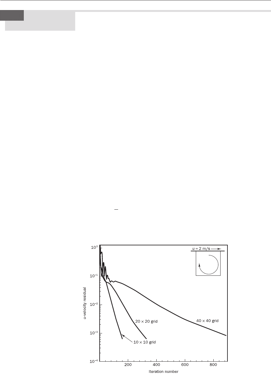
To examine the relationship between the convergence rate of an iterative

method and the number of grid cells in a problem we consider a simple

two-dimensional cavity-driven ﬂow. The inset of Figure 7.5 shows that the

computational domain is a square cavity with a size of 1 cm × 1 cm. The lid

of the cavity is moving with a velocity of 2 m/s in the positive x-direction.

The ﬂuid in the cavity is air and the ﬂow is assumed to be laminar. We use a

line-by-line iterative solver to compute the solution on three different grids

with 10 × 10, 20 × 20 and 40 × 40 cells.

To obtain a measure of the closeness to the true solution of an intermedi-

ate solution in an iteration sequence we use the residual deﬁned in (7.26) for

the ith equation. The average residual Ö over all n equations in the system

(i.e. an average over all the control volumes in the computational domain

of a ﬂow problem) is a useful indicator of iterative convergence for a given

problem:

Ö =|r

| (7.30)

If the iteration process is convergent the average residual Ö should tend to

zero, since all contributing residuals r

→ 0 as k →∞. The average residual

∑

i=1

Multigrid

techniques

7.7

Figure 7.5 Residual reduction

pattern with a line-by-line

iterative solver using different

grid resolutions

ANIN_C07.qxd 29/12/2006 04:48PM Page 229

for a given solution parameter, e.g. the u-velocity component, is usually

normalised to make it easier to interpret its value from case to case and to

compare it with residuals relating to other solution parameters (e.g. v- or

w-velocity or pressure, which may each have very different magnitudes).

The most common normalisation is to consider the ratio of the average

residual after k iterations and its value at the ﬁrst iteration:

(k)

norm

= (7.31)

In Figure 7.5 we have plotted the normalised residual of the u-momentum

equation against the iteration number. The solution is aborted when the

normalised residuals for all solution variables (velocity and pressure in this

case) fall below 10

−3

. We note that the 10 × 10 mesh solution converges in

161 iterations, whereas the 20 × 20 and 40 × 40 mesh solutions take 331 and

891 iterations to converge, respectively. Within the CFD code it is possible

to improve the convergence rate by adjusting solution parameters, including

relaxation parameters, but for the sake of consistency all solution parameters

were kept constant. The pattern of residual reduction is evident from the

diagram. After a rapid initial reduction of the residuals their rate of decrease

settles to a more modest ﬁnal value. It is also clear that the ﬁnal conver-

gence rate is lowest for the ﬁnest mesh. If we tried an even ﬁner mesh,

it would take even longer to converge.

Multigrid concept

To simplify the explanation of the multigrid method we use matrix notation

and ﬁrst revisit the deﬁnition of the residual. Consider the following system

of equations arising from the ﬁnite volume discretisation of a conservation

equation on a ﬂow domain:

A.x= b (7.32)

The vector x is the true solution of system (7.32).

If we solve this system with an iterative method we obtain an intermediate

solution y after some unspeciﬁed number of iterations. This intermediate

solution does not satisfy (7.32) exactly and, as before, we deﬁne the residual

vector r as follows:

A.y= b − r (7.33)

We can also deﬁne an error vector e as the difference between the true solu-

tion and the intermediate solution:

e = x − y (7.34)

Subtracting (7.33) from (7.32) gives the following relationship between the

error vector and the residual vector:

A.e= r (7.35)

The residual vector can be easily calculated at any stage of the iteration pro-

cess by substituting the intermediate solution into (7.33). We can imagine

using an iterative process to solve system (7.35) and obtain the error vector.

For this it might be useful to write the system in the iteration matrix form:

(k)

= T.e

(k−1)

+ c (7.36a)

(k)

(1)

230 CHAPTER 7 SOLUTION OF DISCRETISED EQUATIONS

ANIN_C07.qxd 29/12/2006 04:48PM Page 230

7.7 MULTIGRID TECHNIQUES 231

Since the coefﬁcient matrix A is the same for systems (7.32) and (7.35), the

coefﬁcients T

of the iteration matrix are equal to those of the chosen itera-

tion method, i.e. the Jacobi method or Gauss–Seidel method without or with

relaxation. The elements of the constant vector are, however, different:

= (7.36b)

In practice, if we tried to solve system (7.35) using the same iteration method

as we used for the original system (7.32) we would not ﬁnd that this

made any difference in terms of convergence rate. However, system (7.35) is

important, because it shows how the error propagates from one iteration to

the next. Moreover, its equivalent (7.36) highlights the crucial role played by

the iteration matrix. As we saw earlier when we introduced the relaxation

technique, the properties of the iteration matrix determine the rate of error

propagation and, hence, the rate of convergence.

These properties have been extensively studied along with the math-

ematical behaviour of the error propagation as a function of the iterative

technique, mesh size, discretisation scheme etc. It has been established that

the solution error has components with a range of wavelengths that are

multiples of the mesh size. Iteration methods cause rapid reduction of error

components with short wavelengths up to a few multiples of the mesh size.

However, long-wavelength components of the error tend to decay very

slowly as the iteration count increases.

This error behaviour explains the observed trends in Figure 7.5. For the

coarse mesh, the longest possible wavelengths of error components (i.e. those

of the order of the domain size) are just within the short-wavelength range

of the mesh and, hence, all error components reduce rapidly. On the ﬁner

meshes, however, the longest error wavelengths are progressively further

outside the short-wavelength range for which decay is rapid.

Multigrid methods are designed to exploit these inherent differences of

the error behaviour and use iterations on meshes of different size. The short-

wavelength errors are effectively reduced on the ﬁnest meshes, whereas the

long-wavelength errors decrease rapidly on the coarsest meshes. Moreover,

the computational cost of iterations is larger on ﬁner meshes than on coarse

meshes, so the extra cost due to iterations on the coarse meshes is offset by

the beneﬁt of much improved convergence rate.

7.7.1 An outline of a multigrid procedure

We now give a short description of the principles of a two-stage multigrid

procedure:

Step 1: Fine grid iterations. Perform iterations on the ﬁnest grid with mesh

spacing h to generate an intermediate solution y

to system A

. x = b with

true solution vector x. The number of iterations is chosen sufﬁciently large

that the short-wavelength oscillatory component of the error is effectively

reduced, but no attempt is made to eliminate the long-wavelength error

component. The residual vector r

for the solution on this mesh satisﬁes

= b − A

. y

(see equation (7.33)) and the error vector e

is given by

= x − y

(see equation (7.34)). We have also established that the error and

residual are related as follows: A

. e

= r

(see equation (7.35)).

ANIN_C07.qxd 29/12/2006 04:48PM Page 231

Step 2: Restriction. The solution is transferred from the ﬁne mesh with spac-

ing h onto a coarse mesh with spacing ch, where c > 1. Due to the larger mesh

spacing of the coarse mesh the long-wavelength error (on the ﬁne mesh)

appears as a short-wavelength error on the new mesh and will reduce rapidly.

The process of transferring can be simpliﬁed if we use a coarse mesh with

twice the mesh spacing of the ﬁne mesh. Instead of solving for the solution

vector y

we work with the error equation A

. e

= r

on the coarse mesh

starting with an initial guess of e

= 0. To perform the solution process we

need values of the residual vector and the matrix of coefﬁcients. Given the

values of r

on the ﬁne mesh we must use a suitable averaging procedure to

ﬁnd the residual vector r

on the coarse mesh. The coefﬁcients of matrix A

can be recomputed from scratch on the coarser mesh or evaluated from the

ﬁne mesh coefﬁcient matrix A

using some form of averaging or interpola-

tion technique. The cost per iteration on the coarser mesh is small, so we

can afford to perform an adequate number of iterations to get a converged

solution of the error vector e

Step 3: Prolongation. After obtaining the converged solution of error vector

for the coarse mesh we need to transfer it back to the ﬁne mesh, but note

that we have fewer data than points in the ﬁne mesh. We use a convenient

interpolation operator (e.g. linear interpolation) to generate values for the

prolonged error vector e′

at intermediate points in the ﬁne mesh.

Step 4: Correction and ﬁnal iterations. Once we have calculated the prolonged

error vector e′

we may correct the intermediate ﬁne grid solution: y

improved

+ e′

. Because the long-wavelength error has been eliminated, this

improved solution is closer to the true solution vector x. However, several

approximations were made, so we perform a few more iterations with the

improved solution to iron out any errors that may have been introduced

during restriction and prolongation.

The above description is for the two-stage procedure (one ﬁne mesh, one

coarse mesh). In practice, however, the restriction is carried out into a

number of increasingly coarse levels. Then prolongation procedures are also

performed at each stage back to the starting mesh.

7.7.2 An illustrative example

Consider solving a one-dimensional conduction equation for an insulated

metal rod which has internal heat generation. The governing equation is

k + g = 0

The dimensions and other data are as follows: length of the rod is 1 m, cross-

sectional area of the rod is 0.01 m

, thermal conductivity k = 5 W/m.K,

generation g = 20 kW/m

, the ends are at 100°C and 500°C. We are inter-

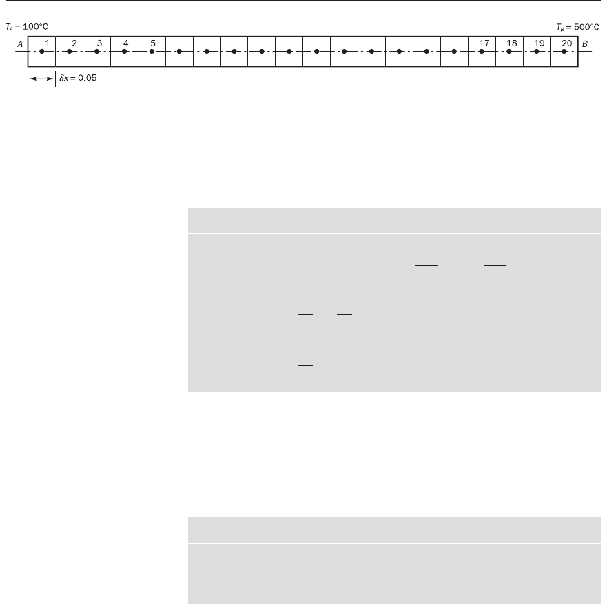
ested in obtaining a solution, say, using a grid of 20 cells giving a spacing of

∆x = 0.05 m, which we name Grid 1.

Figure 7.6 shows Grid 1 along with the boundary conditions marked at

each end. It is not necessary here to describe how discretisation equations

232 CHAPTER 7 SOLUTION OF DISCRETISED EQUATIONS

Example 7.5

Solution

ANIN_C07.qxd 29/12/2006 04:48PM Page 232

7.7 MULTIGRID TECHNIQUES 233

Figure 7.6 The 20 node grids

used to solve the problem –

Grid 1

We use the expressions in Table 7.12 to compile the numerical values

of coefﬁcients in Table 7.13 and to construct the matrix equation A.x= b,

where solution vector x contains the temperatures at the nodes of Grid 1.

Table 7.12 Coefﬁcients of the discretisation equation at each point

Node a

1 (ﬁrst node) 0 qA

x + T

− a

+ a

− S

2, 3,..., 19

(internal nodes)

x 0.0 a

+ a

− S

20 (last node) 0 qA

x + T

− a

+ a

− S

2kA

Table 7.13 Numerical values of the coefﬁcients of the discretisation equation

Node a

1 0 1.0 210 −2.0 3.0

2, 3,..., 19 1.0 1.0 10 0.0 2.0

20 1.0 0 1010 −2.0 3.0

are obtained for this problem; the procedure is similar to Example 4.2.

Table 7.12 gives a summary of coefﬁcients of the discretisation equations at

nodes 1, 2, 3, ..., 20.

The matrix equation is

G 3.0 −1.0 0 . . . 0 JGx

JG210J

H−1.0 2.0 −1.0 . . . 0 KHx

KH10K

H 0 −1.0 2.0 −1.0 . . 0 KHx

KH10K

H .......KH.

K = H .

K (7.37)

H .......KH. KH. K

H ....−1.0 2.0 −1.0KHx

KH10K

I .....−1.0 3.0LIx

LI1010L

The matrix of coefﬁcients is tri-diagonal, so we can use the TDMA to obtain

a solution in a single pass. The result is given in Table 7.14 to enable later

veriﬁcation of the multigrid solution.

ANIN_C07.qxd 29/12/2006 04:48PM Page 233

Step 1: Fine grid iterations

We use the Gauss–Seidel iteration (7.20) to solve these equations. We

simply initialise the temperature to 150°C everywhere as an initial guess to

start the iterative process (a ﬁeld closer to the ﬁnal solution will not highlight

the beneﬁt of the method). The solution vector y

after ﬁve Gauss–Seidel

iterations is shown below:

JG116.755J

KH141.994K

KH160.427K

H . K

(7.38)

H . KH. K

KH394.392K

LI468.130L

The residual vector r

= b − A

. y

at this stage is

JG210JG3.0 −1.0 0 . . . 0 JGy

JG1.728J

KH10KH−1.0 2.0 −1.0 . . . 0 KHy

KH3.193K

KH10KH0 −1.0 2.0 −1.0 . . 0 KHy

KH4.658K

H . K

−

H .......KH. K

H . K

H . KH. KH.......KH. KH. K

KH10KH.. ..−1.0 2.0 −1.0KHy

KH7.461K

LI1010LI.....−1.0 3.0LIy

LI0.000L

The total r.m.s. residual value is 14.951. If the iteration process is continued

the residual vector will reduce slowly until the convergence criterion is

achieved. Figure 7.9 at the end of this section shows the pattern of conver-

gence for the Gauss–Seidel iteration. Using a sum of r.m.s. residuals less

than 10

−6

as the convergence criterion, the ﬁnal solution is achieved after 664

iterations. The converged solution is of course indistinguishable from the

TDMA solution in Table 7.14.

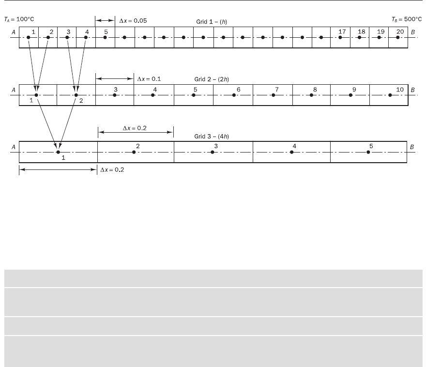
Step 2: Restriction

To apply the multigrid method we have to construct a coarse grid ﬁrst. The

simplest method is to construct a grid which has half the number of cells.

Figure 7.7 shows the ﬁne mesh and the proposed coarse meshes drawn one

beneath the other. The ﬁrst coarse mesh uses 10 cells with a spacing of 0.1 m

and is named Grid 2. The next coarse mesh – Grid 3 – consists of 5 cells with

a spacing of 0.2 m.

If the ﬁne grid mesh spacing is h, a mesh using half the number of

cells would have a mesh spacing of 2h. In the multigrid literature the mesh

spacing is indicated by means of superscripts. In this notation the residual

vector we have on the ﬁne mesh is r

234 CHAPTER 7 SOLUTION OF DISCRETISED EQUATIONS

Table 7.14 The TDMA solution

Grid 1 – Temperature at nodes

1 2 3 4 5 6 7 8 9 1011121314151617181920

160 270 370 460 540 610 670 720 760 790 810 820 820 810 790 760 720 670 610 540

ANIN_C07.qxd 29/12/2006 04:48PM Page 234

7.7 MULTIGRID TECHNIQUES 235

Figure 7.7 Grids used to solve

the problem

Table 7.15 Fine mesh and coarse mesh residuals showing restriction process of transfer from ﬁne Grid 1 to coarse Grid 2

Fine mesh (Grid 1) residuals – (r

)

1 2 3 4 5 67891011121314151617 18 19 20

1.728 3.193 4.658 5.976 7.075 . . . . .......33.962 22.385 7.461 0.000

Coarse mesh (Grid 2) residuals – after restriction (r

)

123456789 10

2.460 5.317 7.506 . . . . . 28.173 3.731

In matrix form the Grid 2 residual vector after ‘restriction’ is

JG2.460J

KH5.317K

KH7.506K

H . K

H . KH. K

KH28.173K

LI3.730L

Note that we have only 10 values now. The error in the coarse mesh satisﬁes

the equation A

. e

= r

. We have calculated the vector r

, but we also

need the matrix A

to solve this equation to obtain e

. In the multigrid

literature there are numerous techniques which use elegant interpolation

operators to evaluate A

. For this example problem we do not interpolate

the coefﬁcient matrix, but calculate the coefﬁcients of the coarse grid matrix

exactly using the expressions in Table 7.12. Thus, we obtain the following

matrix equation for the error vector e

Now we need to interpolate the residual vector from a ﬁne grid to a coarse

grid. Since the nodes of Grid 2 are exactly mid-way between those of Grid 1

we can interpolate by simple averaging of r

to obtain the residual vector r

for the coarse grid. The values are summarised in Table 7.15. Note that only

3 decimal places of the actual numbers are shown in the table. As mentioned

earlier, this transfer process is known as ‘restriction’.

ANIN_C07.qxd 29/12/2006 04:48PM Page 235

G 1.5 −0.5 0 . . . 0JGe

JG2.460J

H−0.5 1.0 −0.5 0 . . 0KHe

KH5.317K

H 0 −0.5 1.0 −0.5 . . 0KHe

KH7.506K

H .......KH . K

H . K

(7.39)

H .......KH . KH. K

H ....−0.5 1.0 −0.5KHe

KH28.173K

I .....−0.5 1.5LIe

LI3.730L

We now solve system (7.39) with an initial guess of e

= (0, 0, 0, ..., 0)

using the Gauss–Seidel iteration procedure. Since the iterations are now

on a coarser mesh, the rate of residual reduction is faster and the cost per

iteration is much lower. After 10 iterations on this coarse mesh we obtain the

error vector e

on the ﬁrst coarse mesh (Grid 2) as

JG19.156J

KH58.310K

KH96.049K

H . K

(7.40)

H . KH . K

KH158.591K

LI55.351L

Since we have only performed 10 iterations this solution is partially converged

and there will be a residual: <

= r

at start

− A

. e

. Its values are given in

Table 7.16 along with interpolated Grid 3 residuals r

after restriction.

236 CHAPTER 7 SOLUTION OF DISCRETISED EQUATIONS

Table 7.16 Residuals on Grid 2 and restricted residuals on Grid 3

Coarse mesh (Grid 2) residuals >

1 2 3 456789 10

2.881 4.609 5.929 .....0.91920.000

Coarse mesh (Grid 3) residuals r

– after restriction

12345

3.745 6.277 6.204 3.615 0.459

Now the residuals <

have been transferred to an even coarser grid with

ﬁve nodes (see Figure 7.7) to yield residual r

. Then we solve for the error

on Grid 3 using the system of equations A

. e

= r

, where the co-

efﬁcients of A

are again calculated from scratch using the expressions in

Table 7.12. As the cost per iteration is very low we can afford to do more

iterations on Grid 3 to achieve very effective error reduction. After 10 itera-

tions we get the solution in Table 7.17 for error vector e

Table 7.17

Grid 3 – solution (error vector e

on Grid 3)

12345

23.408 55.831 63.731 47.205 16.348

This coarsening procedure could be continued, but in this illustrative

example we stop the process of restriction at the ﬁve-node grid.

ANIN_C07.qxd 29/12/2006 04:48PM Page 236