Versteeg H., Malalasekra W. An Introduction to Computational Fluid Dynamics: The Finite Volume Method
Подождите немного. Документ загружается.


8.2 ONE-DIMENSIONAL UNSTEADY HEAT CONDUCTION 247
ρ
c > (8.13a)
or
∆t <
ρ
c (8.13b)
This inequality sets a stringent maximum limit to the time step size and rep-
resents a serious limitation for the explicit scheme. It becomes very expen-
sive to improve spatial accuracy because the maximum possible time step
needs to be reduced as the square of ∆x. Consequently, this method is not
recommended for general transient problems. Explicit schemes with greater
formal accuracy than the above one have been designed. Examples are the
Richardson and DuFort–Frankel methods, which use temperatures at more
than two time levels. These methods also have fewer stability restrictions
than the ordinary explicit method. Details of such schemes can be found in
Abbot and Basco (1990), Anderson et al (1984) and Fletcher (1991). Never-
theless, provided that the time step size is chosen with care, the explicit
scheme described above is efficient for simple conduction calculations. This
will be illustrated through an example in section 8.3.
8.2.2 Crank---Nicolson scheme
The Crank–Nicolson method results from setting
θ
= 1/2 in equation (8.11).
The source term is linearised as b = S
u
+
1
–
2
S
P
T
P
+
1
–
2
S
P
T
o
P
. Now the discre-
tised unsteady heat conduction equation is
a
P
T
P
= a
E
+ a
W
+ a
o
P
−− T
o
P
+ S
u
+ S
p
T
o
P
(8.14)
where
a
P
= (a
W
+ a
E
) + a
o
P
− S
p
and
a
o
P
=
ρ
c
a
W
a
E
k
e
δ
x
PE
k
w
δ
x
WP
∆x
∆t
1
2
1
2
1
2
J
K
L
a
W
2
a
E
2
G
H
I
J
K
L
T
W
+ T
o
W
2
G
H
I
J
K
L
T
E
+ T
o
E
2
G
H
I
(∆x)
2
2k
2k
∆x
∆x
∆t
ANIN_C08.qxd 29/12/2006 04:38PM Page 247

248 CHAPTER 8 THE FINITE VOLUME METHOD FOR UNSTEADY FLOWS
Since more than one unknown value of T at the new time level is present
in equation (8.14) the method is implicit, and simultaneous equations for
all node points need to be solved at each time step. Although schemes with
1
–
2
≤
θ
≤ 1, including the Crank–Nicolson scheme, are unconditionally stable
for all values of the time step (Fletcher, 1991), it is more important to ensure
that all coefficients are positive for physically realistic and bounded results.
This is the case if the coefficient of T
o
P
satisfies the following condition:
a
o
P
>
which leads to
∆t <
ρ
c (8.15)
This time step limitation is only slightly less restrictive than (8.13) associated
with the explicit method. The Crank–Nicolson method is based on central
differencing and hence it is second-order accurate in time. With sufficiently
small time steps it is possible to achieve considerably greater accuracy than
with the explicit method. The overall accuracy of a computation depends
also on the spatial differencing practice so the Crank–Nicolson scheme is
normally used in conjunction with spatial central differencing.
8.2.3 The fully implicit scheme
When the value of
θ
is set equal to 1 we obtain the fully implicit scheme. Now
the source term is linearised as b = S
u
+ S
P
T
P
. The discretised equation is
a
P
T
P
= a
W
T
W
+ a
E
T
E
+ a
o
P
T
o
P
+ S
u
(8.16)
where
a
P
= a
o
P
+ a
W
+ a
E
− S
p
and
a
o
P
=
ρ
c
with
a
W
a
E
Both sides of the equation contain temperatures at the new time step, and
a system of algebraic equations must be solved at each time level (see
Example 8.2). The time marching procedure starts with a given initial field
k
e
δ
x
PE
k
w
δ
x
WP
∆x
∆t
∆x
2
k
J
K
L
a
E
+ a
W
2
G
H
I
ANIN_C08.qxd 29/12/2006 04:38PM Page 248

8.3 ILLUSTRATIVE EXAMPLES 249
of temperatures T
O
. The system of equations (8.16) is solved after selecting
time step ∆t. Next the solution T is assigned to T
O
and the procedure is
repeated to progress the solution by a further time step.
It can be seen that all coefficients are positive, which makes the implicit
scheme unconditionally stable for any size of time step. Since the accuracy of
the scheme is only first-order in time, small time steps are needed to ensure
the accuracy of results. The implicit method is recommended for general-
purpose transient calculations because of its robustness and unconditional
stability.
We now demonstrate the properties of the explicit and implicit discretisa-
tion schemes by means of a comparison of numerical results for a one-
dimensional unsteady conduction example with analytical solutions to
assess the accuracy of the methods.
A thin plate is initially at a uniform temperature of 200°C. At a certain time
t = 0 the temperature of the east side of the plate is suddenly reduced to 0°C.
The other surface is insulated. Use the explicit finite volume method in con-
junction with a suitable time step size to calculate the transient temperature
distribution of the slab and compare it with the analytical solution at time
(i) t = 40 s, (ii) t = 80 s and (iii) t = 120 s. Recalculate the numerical solution
using a time step size equal to the limit given by (8.13) for t = 40 s and com-
pare the results with the analytical solution. The data are: plate thickness
L = 2 cm, thermal conductivity k = 10 W/m.K and
ρ
c = 10 × 10
6
J/m
3
.K.
The one-dimensional transient heat conduction equation is
ρ
c = k (8.17)
and the initial conditions are
T = 200 at t = 0
and the boundary conditions are
= 0 at x = 0, t > 0
T = 0 at x = L, t > 0
The analytical solution is given in Özivik (1985) as
= exp(−
αλ
2
n
t) cos(
λ
n
x) (8.18)
where
λ
n
= and
α
= k/
ρ
c
The numerical solution with the explicit method is generated by dividing
the domain width L into five equal control volumes with ∆x = 0.004 m. The
resulting one-dimensional grid is shown in Figure 8.2.
(2n − 1)
π
2L
(−1)
n+1
2n − 1
∞
∑
n=1
4
π
T(x, t)
200
∂
T
∂
x
D
E
F
∂
T
∂
x
A
B
C
∂
∂
x
∂
T
∂
t
Illustrative
examples
8.3
Example 8.1
Solution
ANIN_C08.qxd 29/12/2006 04:38PM Page 249

250 CHAPTER 8 THE FINITE VOLUME METHOD FOR UNSTEADY FLOWS
Figure 8.2 Geometry for
Example 8.1
The discretised form of governing equation (8.17) for an internal control
volume using the explicit method is given by (8.12). Control volumes 1 and
5 adjoin boundaries, so the links are cut in the direction of the boundary and
the boundary fluxes are included in the source terms. At the control volume
1, the west boundary is insulated: hence the flux across that boundary is zero.
We modify equation (8.9) where the physics can be most easily discerned.
The discretised equation at node 1 becomes
ρ
c ∆x = (T
o
E
− T
o
P
) − 0 (8.19)
For time t > 0, the temperature of the east boundary of control volume 5 is
constant (say T
B
). The discretised equation at node 5 becomes
ρ
c ∆x = (T
B
− T
o
P
) − (T
o
P
− T
o
W
) (8.20)
All discretised equations can now be written in standard form:
a
P
T
P
= a
W
T
o
W
+ a
E
T
o
E
+ [a
o
P
− (a
W
+ a
E
)]T
o
P
+ S
u
(8.21)
where
a
P
= a
o
P
=
ρ
c
and
Node a
W
a
E
S
u
10k/∆x 0
2, 3, 4 k/∆xk/∆x 0
5 k/∆x 0(T
B
− T
o
P
)
The time step for the explicit method is subject to the condition that
∆t <
∆t <
∆t < 8 s
10 × 10
6
(0.004)
2
2 × 10
ρ
c(∆x)
2
2k
2k
∆x
∆x
∆t
J
K
L
k
∆x
G
H
I
J
K
L
k
∆x/2
G
H
I
(T
P
− T
o
P
)
∆t
J
K
L
k
∆x
G
H
I
(T
P
− T
o
P
)
∆t
ANIN_C08.qxd 29/12/2006 04:38PM Page 250

8.3 ILLUSTRATIVE EXAMPLES 251
Let us select ∆t = 2 s. Substituting numerical values we have
==2500
ρ
c = 10 × 10
6
×=20000
After substitution of numerical values and some simplification the discretisa-
tion equations for the various nodes are
Node 1: 200T
P
= 25T
o
E
+ 175T
o
P
Nodes 2–4: 200T
P
= 25T
o
W
+ 25T
o
E
+ 150T
o
P
(8.22)
Node 5: 200T
P
= 25T
o
W
+ 125T
o
P
Starting with the initial condition where all the nodes are at a temperature
of 200°C, the solution at each time step is obtained using equations (8.22).
Although the calculations are not complicated, their number is large and
they are most effectively carried out by a computer program. Table 8.1 gives
a sample of the calculations for the first two time steps.
0.004
2
∆x
∆t
10
0.004
k
∆x
Table 8.1 Specimen calculations for the explicit method
Time Node 1 Node 2 Node 3 Node 4 Node 5
t = 0 s T
0
1
= 200 T
0
2
= 200 T
0
3
= 200 T
0
4
= 200 T
0
5
= 200
200T
1
1
= 25 × 200 200T
1
2
= 25 × 200 200T
1
3
= 25 × 200 200T
1
4
= 25 × 200 200T
1
5
= 25 × 200
+ 175 × 200 + 25 × 200 + 25 × 200 + 25 × 200 + 125 × 200
+ 150 × 200 + 150 × 200 + 150 × 200
t = 2 s T
1
1
= 200 T
1
2
= 200 T
1
3
= 200 T
1
4
= 200 T
1
5
= 150
200T
2
1
= 25 × 200 200T
2
2
= 25 × 200 200T
2
3
= 25 × 200 200T
2
4
= 25 × 200 200T
2
5
= 25 × 200
+ 175 × 200 + 25 × 200 + 25 × 200 + 25 × 150 + 125 × 150
+ 150 × 200 + 150 × 200 + 150 × 200
t = 4 s T
2
1
= 200 T
2
2
= 200 T
2
3
= 200 T
2
4
= 193.75 T
2
5
= 118.75
Note: Subscripts denote the node number, superscripts denote the time step
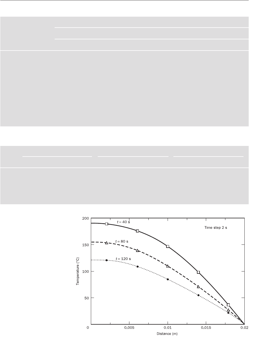
Table 8.2 shows the results for 10 consecutive time steps and Table 8.3
shows the numerical and analytical results at times 40, 80 and 120 s. As can
be seen from the error analysis, the results are in good agreement with the
analytical solution. Figure 8.3 shows the comparison in a graphical form.
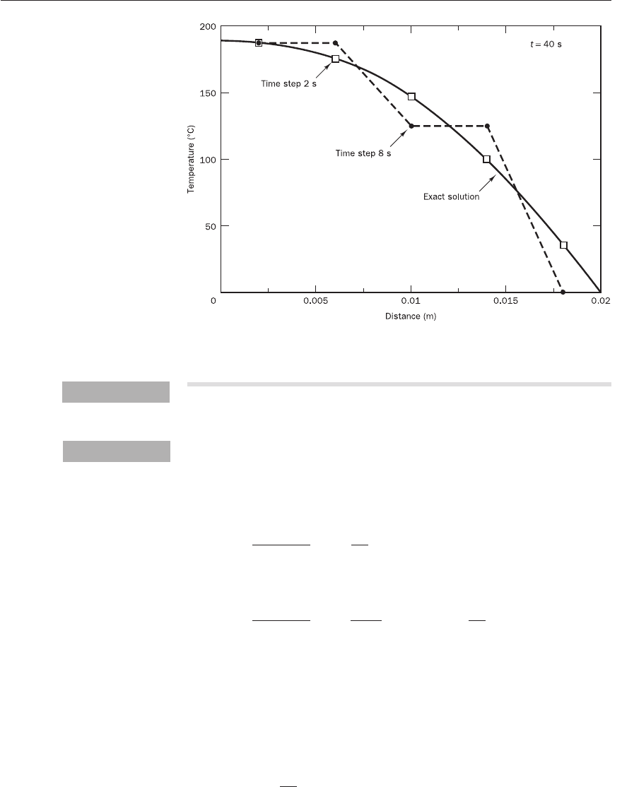
Figure 8.4 shows the solution for time t = 40 s with a time step of 8 s. The
previous result with a step size of 2s and the exact solution are also shown for
comparison. We conclude that a time step equal to the limiting value of 8 s
gives a very inaccurate and unrealistic numerical solution that oscillates
about the exact solution.
ANIN_C08.qxd 29/12/2006 04:38PM Page 251
252 CHAPTER 8 THE FINITE VOLUME METHOD FOR UNSTEADY FLOWS
Figure 8.3 Comparison of
numerical and analytical
solutions at different times
Table 8.2 Results for Example 8.1 (explicit method)
Node number
Time
12345
step Time (s) x = 0.0 x = 0.002 x = 0.006 x = 0.01 x = 0.014 x = 0.016 x = 0.018
0 0 200 200 200 200 200 200 200
1 2 200 200 200 200 200 150 0
2 4 200 200 200 200 193.75 118.75 0
3 6 200 200 200 199.21 185.16 98.43 0
4 8 200 200 199.9 197.55 176.07 84.66 0
5 10 199.98 199.98 199.62 195.16 167.33 74.92 0
6 12 199.94 199.94 199.11 192.24 159.26 67.74 0
7 14 199.83 199.83 198.35 188.98 151.94 62.24 0
8 16 199.65 199.65 197.36 185.52 145.36 57.89 0
9 18 199.37 199.37 196.17 181.98 139.45 54.35 0
10 20 198.97 198.97 194.79 178.44 134.12 51.40 0
Table 8.3
Time = 40 s Time = 80 s Time = 120 s
Node Numerical Analytical % error Numerical Analytical % error Numerical Analytical % error
1 188.64 188.39 −0.13 153.33 152.65 −0.43 120.53 119.87 −0.55
2 176.41 175.76 −0.36 139.05 138.36 −0.50 108.82 108.21 −0.56
3 148.29 147.13 −0.79 111.29 110.63 −0.59 86.47 85.96 −0.58
4 100.76 99.50 −1.26 72.06 71.56 −0.69 55.58 55.25 −0.60
5 35.94 35.38 −1.57 24.96 24.77 −0.75 19.16 19.05 −0.59
ANIN_C08.qxd 29/12/2006 04:38PM Page 252
8.3 ILLUSTRATIVE EXAMPLES 253
Solve the problem of Example 8.1 again using the fully implicit method and
compare the explicit and implicit method solutions for a time step of 8 s.
Let us use the same grid arrangement as in Figure 8.2. The fully implicit
method describes events at internal control volumes 2, 3 and 4 by means of
discretised equation (8.16). Boundary control volumes 1 and 5 again need
special treatment. Upon incorporating the boundary conditions into equa-
tion (8.9) we get for node 1
ρ
c ∆x = (T
E
− T
P
) − 0 (8.23)
and for node 5
ρ
c ∆x = (T
B
− T
P
) − (T
P
− T
W
) (8.24)
The discretised equations are written in standard form:
a
P
T
P
= a
W
T
W
+ a
E
T
E
+ a
o
P
T
o
P
+ S
u
(8.25)
where
a
P
= a
W
+ a
E
+ a
o
P
− S
P
and
a
o
P
=
ρ
c
and
∆x
∆t
J
K
L
k
∆x
G
H
I
J
K
L
k
∆x/2
G
H
I
(T
P
− T
o
P
)
∆t
J
K
L
k
∆x
G
H
I
(T
P
− T
o
P
)
∆t
Figure 8.4 Comparison of
results obtained using different
time step values
Example 8.2
Solution
ANIN_C08.qxd 29/12/2006 04:38PM Page 253

254 CHAPTER 8 THE FINITE VOLUME METHOD FOR UNSTEADY FLOWS
Node a
W
a
E
S
P
S
u
10k/∆x 00
2, 3, 4 k/∆xk/∆x 00
5 k/∆x 0 − T
B
Although the implicit method permits large values for the time step ∆t, we
will use reasonably small time steps of 2 s to ensure good accuracy. The grid
spacing and other data are as before so again we have
==2500
ρ
c = 10 × 10
6
×=20000
After substitution of numerical values and the necessary simplification the
discretised equations for the various nodes are
Node 1: 225T
P
= 25T
E
+ 200T
o
P
Nodes 2–4: 250T
P
= 25T
W
+ 25T
E
+ 200T
o
P
Node 5: 275T
P
= 25T
W
+ 200T
o
P
+ 50T
B
Noting that T
B
= 0, the set of equations to be solved at each time step is
G225 −25000JGT
1
JG200T
o
1
J
H−25 250 −25 0 0KHT
2
KH200T
o
2
K
H 0 −25 250 −25 0KHT
3
K = H200T
o
3
K (8.26)
H 00−25 250 −25KHT
4
KH200T
o
4
K
I 000−25 275LIT
5
LI200T
o
5
L
The matrix form emphasises that the equations for each point contain
unknown neighbouring temperatures. The explicit scheme involves a
straightforward evaluation of a single algebraic equation to find each new
nodal temperature, but the fully implicit method requires the (more expen-
sive) solution of system (8.26) at each time level. The values of temperature
at the previous time level are used to calculate the right hand side. Table 8.4
and Figure 8.5 show that the numerical results again compare favourably
with the analytical solution.
0.004
2
∆x
∆t
10
0.004
k
∆x
2k
∆x
2k
∆x
Table 8.4
Time = 40 s Time = 80 s Time = 120 s
Node Numerical Analytical % error Numerical Analytical % error Numerical Analytical % error
1 187.38 188.38 0.51 153.72 152.65 −0.70 121.52 119.87 −1.42
2 176.28 175.76 −0.29 139.79 138.36 −1.03 109.78 108.21 −1.24
3 150.04 147.13 −1.97 112.38 110.63 −1.57 87.33 85.96 −1.59
4 103.69 99.50 −4.20 73.09 71.56 −2.13 56.20 55.25 −1.71
5 37.51 35.38 −6.02 25.38 24.77 −2.46 19.39 19.05 −1.78
ANIN_C08.qxd 29/12/2006 04:38PM Page 254
8.3 ILLUSTRATIVE EXAMPLES 255
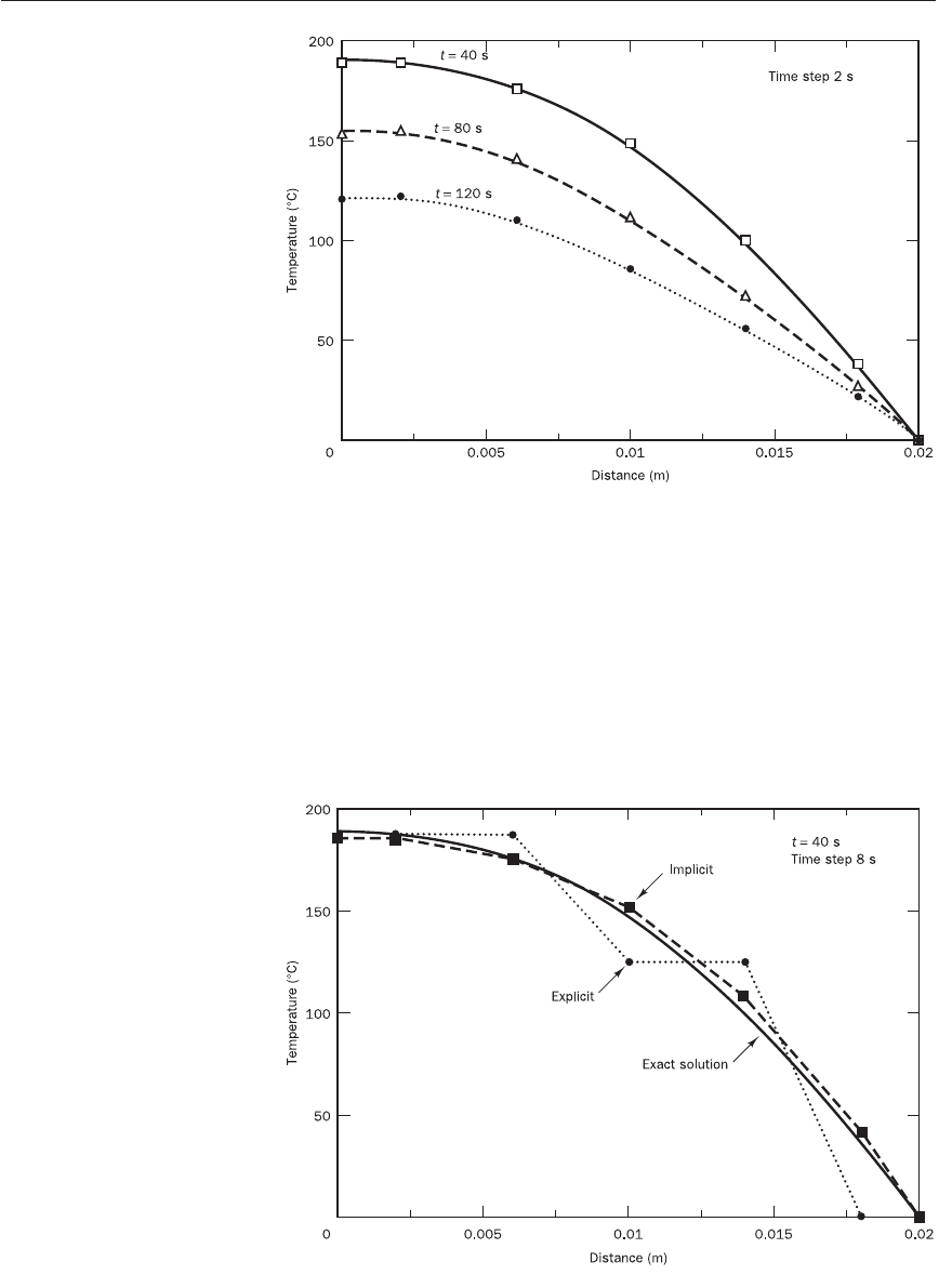
In Figure 8.6 we give the solution at t = 40 s obtained using the implicit
and explicit method with a time step of 8 s along with the analytical solution.
Whereas the explicit method gives unrealistic oscillations at this step size,
the implicit method gives results that are in reasonable agreement with
the exact solution. This clearly illustrates a key advantage of the implicit
method, which tolerates much larger time steps. However, we stress that
good solution accuracy can, of course, only be achieved with small time
steps.
Figure 8.5 Comparison of
numerical results with the
analytical solution (implicit
method)
Figure 8.6 Comparison of
implicit and explicit solutions
for ∆t = 8 s
ANIN_C08.qxd 29/12/2006 04:38PM Page 255

256 CHAPTER 8 THE FINITE VOLUME METHOD FOR UNSTEADY FLOWS
The fully implicit method is recommended for general-purpose CFD com-
putations on the grounds of its superior stability. We now quote its extension
to calculations in two and three space dimensions. Transient diffusion in
three dimensions is governed by
ρ
c =Γ+Γ+Γ+S (8.27)
A three-dimensional control volume is considered for the discretisation. The
resulting equation is
a
P
φ
P
= a
W
φ
W
+ a
E
φ
E
+ a
S
φ
S
+ a
N
φ
N
+ a
B
φ
B
+ a
T
φ
T
+ a
o
P
φ
o
P
+ S
u
(8.28)
where
a
P
= a
W
+ a
E
+ a
S
+ a
N
+ a
B
+ a
T
+ a
o
P
− S
P
a
o
P
=
ρ
c
The neighbouring coefficients are a
W
, a
E
in one-dimensional problems,
and a
W
, a
E
, a
S
, a
N
in two and a
W
, a
E
, a
S
, a
N
, a
B
, a
T
in three dimensions;
b = (S
u
+ S
p
φ
P
) is the linearised source. A summary of the relevant neighbour
coefficients is given below:
a
W
a
E
a
S
a
N
a
B
a
T
1D – – – –
2D – –
3D
The following values for the volume and cell face areas apply in the three cases:
1D 2D 3D
∆V ∆x ∆x∆y ∆x∆y∆z
A
w
= A
e
1 ∆y ∆y∆z
A
n
= A
s
– ∆x ∆x∆z
A
b
= A
t
––∆x∆y
Γ
t
A
t
δ
z
PT
Γ
b
A
b
δ
z
BP
Γ
n
A
n
δ
y
PN
Γ
s
A
s
δ
y
SP
Γ
e
A
e
δ
x
PE
Γ
w
A
w
δ
x
WP
Γ
n
A
n
δ
y
PN
Γ
s
A
s
δ
y
SP
Γ
e
A
e
δ
x
PE
Γ
w
A
w
δ
x
WP
Γ
e
A
e
δ
x
PE
Γ
w
A
w
δ
x
WP
∆V
∆t
D
E
F
∂φ
∂
z
A
B
C
∂
∂
z
D
E
F
∂φ
∂
y
A
B
C
∂
∂
y
D
E
F
∂φ
∂
x
A
B
C
∂
∂
x
∂φ
∂
t
Implicit method
for two- and
three-dimensional
problems
8.4
ANIN_C08.qxd 29/12/2006 04:38PM Page 256