Versteeg H., Malalasekra W. An Introduction to Computational Fluid Dynamics: The Finite Volume Method

Подождите немного. Документ загружается.

All CFD problems are deﬁned in terms of initial and boundary conditions.

It is important that the user speciﬁes these correctly and understands their

role in the numerical algorithm. In transient problems the initial values of all

the ﬂow variables need to be speciﬁed at all solution points in the ﬂow domain.

Since this involves no special measures other than initialising the appropriate

data arrays in the CFD code, we do not need to discuss this topic further.

The present chapter describes the implementation in the discretised equations

of the ﬁnite volume method of the most common boundary conditions:

• inlet

• outlet

• wall

• prescribed pressure

• symmetry

• periodicity (or cyclic boundary condition)

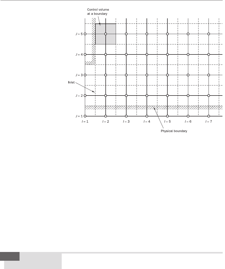
In constructing a staggered grid arrangement we set up additional nodes

surrounding the physical boundary, as illustrated in Figure 9.1. The calcu-

lations are performed at internal nodes only (I = 2 and J = 2 onwards). Two

notable features of the arrangement are (i) the physical boundaries coincide

with scalar control volume boundaries and (ii) the nodes just outside the inlet

of the domain (along I = 1 in Figure 9.1) are available to store the inlet con-

ditions. This enables the introduction of boundary conditions to be achieved

with small modiﬁcations to the discretised equations for near-boundary

internal nodes.

In Chapters 4 and 5 we saw that boundary conditions enter the discretised

equations by suppression of the link to the boundary side and modiﬁcation

of the source terms. The appropriate coefﬁcient of the discretised equation

is set to zero and the boundary side ﬂux – exact or linearly approximated –

is introduced through source terms S

and S

. We will frequently make use

of this device to ﬁx the ﬂux of a variable at a cell face, but we also need a tech-

nique to cope with situations where we need to set the value of a variable at

a node. This can be done by introducing two overwhelmingly large source

terms into the relevant discretised equation. For example, to set the variable

at node P to a value

ﬁx

the following source term modiﬁcation is used in

its discretised equation:

=−10

and S

= 10

ﬁx

(9.1)

With these sources added to the discretised equation we have

+ 10

)

=∑ a

+ 10

ﬁx

(9.2)

Chapter nine Implementation of boundary

conditions

Introduction9.1

ANIN_C09.qxd 29/12/2006 10:01 AM Page 267

The actual magnitude of the number 10

is arbitrary as long as it is very

large compared with all coefﬁcients in the original discretised equation.

Thus if a

and a

are all negligible the discretised equation effectively

states that

ﬁx

(9.3)

which ﬁxes the value of

at P.

In addition to setting the value of a variable at internal nodes this

treatment is also useful for dealing with solid obstacles within a domain by

taking

ﬁx

= 0 (or any other desired value) at nodes within a solid region. The

system of discretised ﬂow equations can be solved as normal without having

to deal with the obstacles separately.

Details of the modiﬁcations needed to implement the listed boundary

conditions will be further explained in the text to follow. We make the

following assumptions: (i) the ﬂow is always subsonic (M < 1), (ii) k–

turbulence modelling is used, (iii) the hybrid differencing method is used

for discretisation and (iv) the SIMPLE solution algorithm is applied.

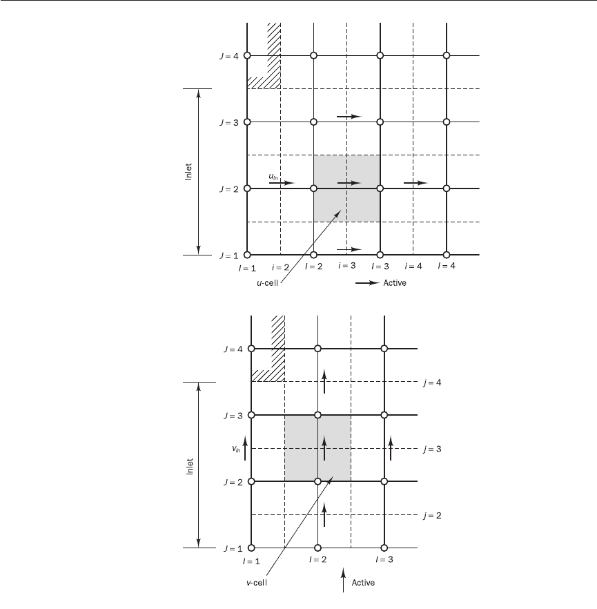
The distribution of all ﬂow variables needs to be speciﬁed at inlet bound-

aries. Here we discuss the case of an inlet perpendicular to the x-direction.

Figures 9.2 to 9.5 show the grid arrangement in the immediate vicinity of an

inlet for u- and v-momentum, scalar and pressure correction equation cells.

The ﬂow direction is assumed to be broadly from the left to the right in the

diagrams. As mentioned, the grid extends outside the physical boundary and

the nodes along the line I = 1 (or i = 2 for u-velocity) are used to store the inlet

values of ﬂow variables (indicated by u

, v

and p′

). Just downstream of

268 CHAPTER 9 IMPLEMENTATION OF BOUNDARY CONDITIONS

Figure 9.1 The grid

arrangement at boundaries

Inlet boundary

conditions

9.2

ANIN_C09.qxd 29/12/2006 10:01 AM Page 268

9.2 INLET BOUNDARY CONDITIONS 269

this extra node we start to solve the discretised equation for the ﬁrst internal

cell, which is shaded.

The diagrams also show the ‘active’ neighbours and cell faces which are

represented in the discretised equation for the shaded cell assuming that

hybrid differencing is used. For instance, in Figure 9.2 the active neighbour

velocities are given by means of arrows and the active face pressures by open

circles. The ﬁgures indicate that all links to neighbouring nodes remain

active for the ﬁrst u-, v- and

-cell, so to accommodate the inlet boundary

condition for these variables it is unnecessary to make any modiﬁcations to

their discretised equations. Figure 9.4 shows that the link with the boundary

side is cut in the discretised pressure correction equation by setting the

boundary side (west) coefﬁcient a

equal to zero. Since the velocity is known

Figure 9.2 u-velocity cell at the

inlet boundary

Figure 9.3 v-velocity cell at the

inlet boundary

ANIN_C09.qxd 29/12/2006 10:01 AM Page 269

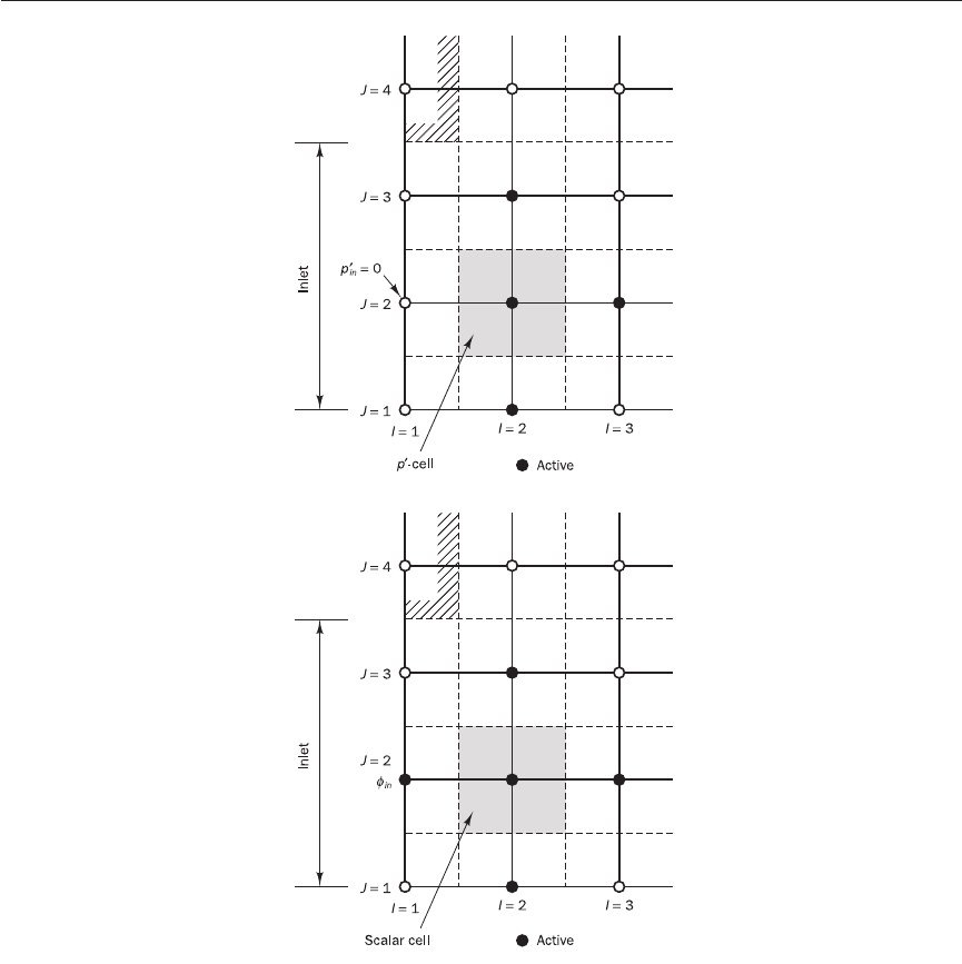
at inlet, it is also not necessary to make a velocity correction here and hence

we have

= u

(9.4)

in the source associated with discretised pressure correction (6.32).

Reference pressure

The pressure ﬁeld obtained by solving the pressure correction equation does

not give absolute pressures (Patankar, 1980). It is common practice to ﬁx the

absolute pressure at one inlet node and set the pressure correction to zero at

that node. Having speciﬁed a reference value, the absolute pressure ﬁeld

inside the domain can now be obtained.

270 CHAPTER 9 IMPLEMENTATION OF BOUNDARY CONDITIONS

Figure 9.4 Pressure correction

cell at the inlet boundary

Figure 9.5 Scalar cell at the

inlet boundary

ANIN_C09.qxd 29/12/2006 10:01 AM Page 270

9.3 OUTLET BOUNDARY CONDITIONS 271

Estimation of k and

εε

at inlet boundaries

The most accurate simulations can only be achieved by supplying measured

inlet values of turbulent kinetic energy k and dissipation rate

. However, if

we perform outline design calculations such data are often not available. In

this case commercial CFD codes often estimate k and

with the approximate

formulae described in section 3.7.2, based on a turbulence intensity – typically

between 1% and 6% – and a length scale.

Inlet boundaries perpendicular to the y-direction

The above procedure is, of course, not restricted to an inlet boundary per-

pendicular to the x-direction. When we have an inlet perpendicular to the

y-direction the velocity component v, for which inlet value v

is available at

j = 2, takes the place of velocity component u and the calculations start

at j = 3. The inlet values of the remaining variables are stored at J = 1 and

solution starts at J = 2. They are otherwise treated as above.

Outlet boundary conditions may be used in conjunction with the inlet

boundary conditions of section 9.2. If the location of the outlet is selected far

away from geometrical disturbances the ﬂow eventually reaches a fully devel-

oped state where no change occurs in the ﬂow direction. In such a region we

can place an outlet surface and state that the gradients of all variables (except

pressure) are zero in the ﬂow direction. It is normally possible to make a

reasonably accurate prediction of the ﬂow direction far away from obstacles.

This gives us the opportunity to locate the outlet surface perpendicular to

the ﬂow direction and take gradients in the direction normal to the outlet

surface equal to zero.

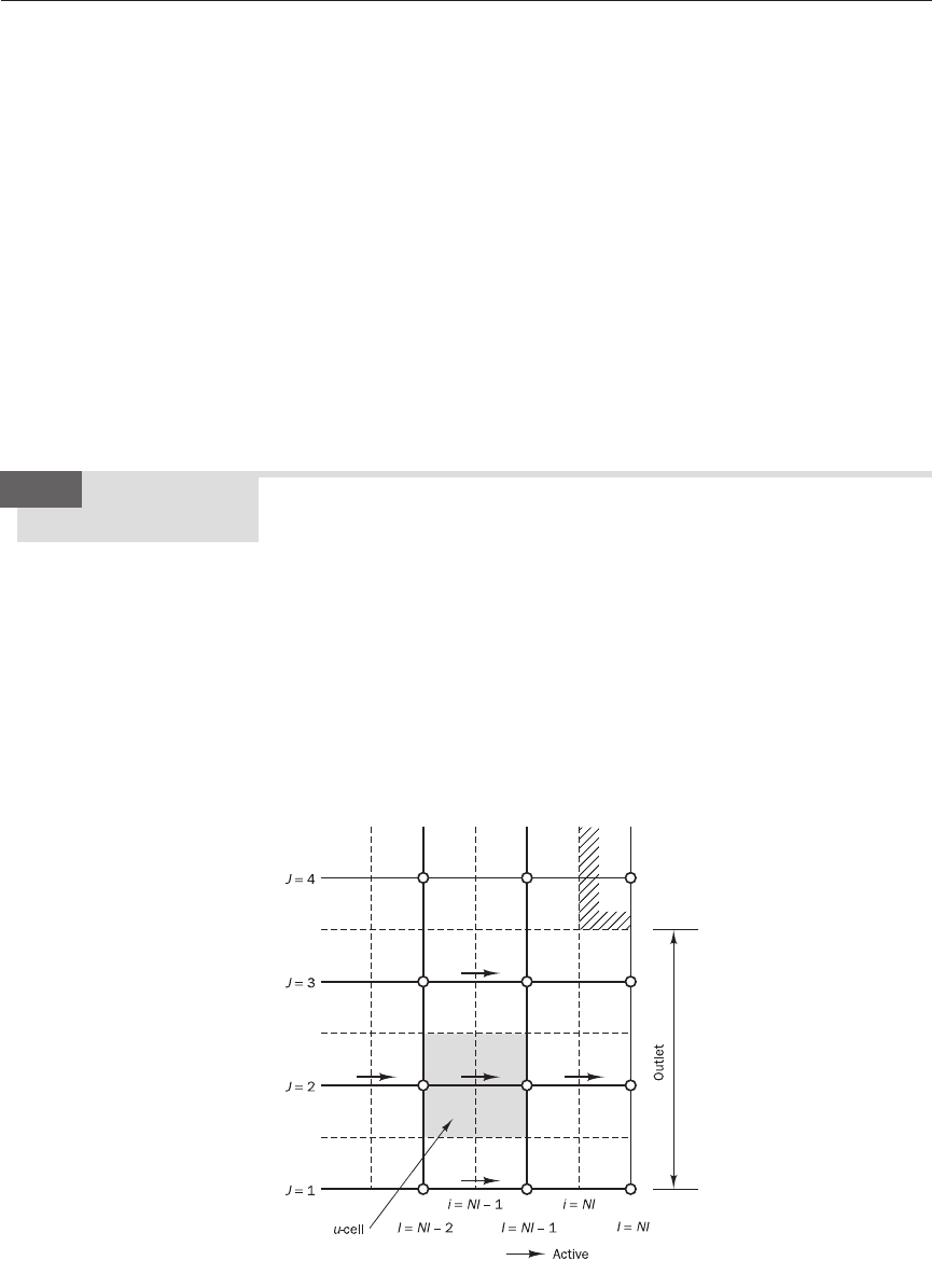
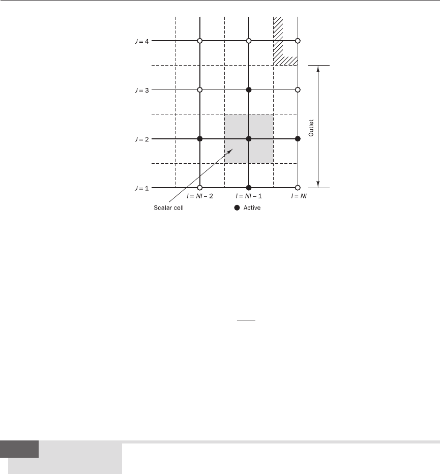
Figures 9.6 to 9.9 show grid arrangements near such an outlet boundary.

We have shaded the last cells upstream of the outlet, for which a discretised

equation is solved, and, as before, highlighted the active neighbours and faces.

Figure 9.6 u-control volume at

an outlet boundary

Outlet boundary

conditions

9.3

ANIN_C09.qxd 29/12/2006 10:01 AM Page 271

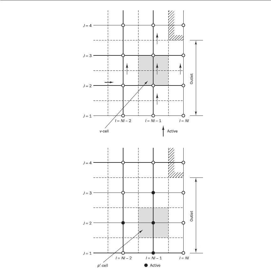
If NI is the total number of nodes in the x-direction, equations are solved

for cells up to I (or i) = NI − 1. Before the relevant equations are solved the

values of ﬂow variables at the next node (NI), just outside the domain, are

determined by extrapolation from the interior on the assumption of zero gradi-

ent at the outlet plane. For the v- and scalar equations this implies setting

NI, j

= v

−

1, j

and

NI, J

−

1, J

. Figures 9.7 and 9.9 show that all links are

active for these variables so their discretised equations can be solved as normal.

Special care should be taken in the case of the u-velocity. Calculation of u

at the outlet plane i = NI by assuming a zero gradient gives

NI, J

= u

NI−1, J

(9.5)

During the iteration cycles of the SIMPLE algorithm there is no guarantee

that these velocities will conserve mass over the computational domain as a

272 CHAPTER 9 IMPLEMENTATION OF BOUNDARY CONDITIONS

Figure 9.7 v-control volume at

an outlet boundary

Figure 9.8 p′-control volume at

an outlet boundary

ANIN_C09.qxd 29/12/2006 10:01 AM Page 272

9.4 WALL BOUNDARY CONDITIONS 273

whole. To ensure that overall continuity is satisﬁed the total mass ﬂux going

out of the domain (M

out

) is ﬁrst computed by summing all the extrapolated

outlet velocities (9.5). To make the mass ﬂux out equal to the mass ﬂux M

coming into the domain all the outlet velocity components u

NI, J

of (9.5) are

multiplied by the ratio M

out

. Thus the outlet plane velocities with the

continuity correction are given by

NI, J

= u

−

1, J

× (9.6)

These values are subsequently used as the east neighbour velocities in the

discretised momentum equations for u

NI−1, J

The velocity at the outlet boundaries is not corrected by means of

pressure corrections. Hence in the discretised p′-equation (6.32) the link

to the outlet boundary side (east) is suppressed by setting a

= 0. The

contribution to the source term in this equation is calculated as normal,

noting that u*

= u

; no additional modiﬁcations are required.

The wall is the most common boundary encountered in conﬁned ﬂuid ﬂow

problems. In this section we consider a solid wall parallel to the x-direction.

Figures 9.10 to 9.12 illustrate the grid details in the near-wall regions for the

u-velocity component (parallel to the wall), for the v-velocity component

(perpendicular to the wall) and for scalar variables.

The no-slip condition (u = v = 0) is the appropriate condition for the

velocity components at solid walls. The normal component of the velocity

can simply be set to zero at the boundary ( j = 2), and the discretised momen-

tum equation at the next v-cell in the ﬂow ( j = 3) can be evaluated without

modiﬁcation. Since the wall velocity is known it is also unnecessary to

perform a pressure correction here. In the discretised p′-equation (6.32) for

the cell nearest to the wall the wall link (south) is, therefore, cut by setting

= 0, and we take v

* = v

in its source term.

out

Figure 9.9 Scalar cell at an

outlet boundary

Wall boundary

conditions

9.4

ANIN_C09.qxd 29/12/2006 10:01 AM Page 273

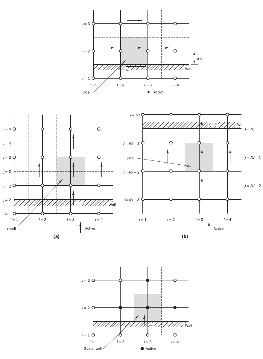
274 CHAPTER 9 IMPLEMENTATION OF BOUNDARY CONDITIONS

Figure 9.10 u-velocity cell at a

wall boundary

Figure 9.11 v-cell at a wall boundary: (a) j = 3 and (b) j = NJ

Figure 9.12 Scalar cell at a wall

boundary

ANIN_C09.qxd 29/12/2006 10:01 AM Page 274

9.4 WALL BOUNDARY CONDITIONS 275

For all other variables special sources are constructed, the precise form

of which depends on whether the ﬂow is laminar or turbulent. In Chapter 3

we studied the multi-layered structure of the near-wall turbulent boundary

layer. Immediately adjacent to the wall we have an extremely thin viscous

sub-layer followed by the buffer layer and the turbulent core. The number

of mesh points required to resolve all the details in a turbulent boundary

layer would be prohibitively large, and normally we employ the ‘wall func-

tions’ introduced in Chapter 3 to represent the effect of the wall boundaries.

The implementation of wall boundary conditions in turbulent ﬂows starts

with the evaluation of

(9.7)

where ∆y

is the distance of the near-wall node P to the solid surface (see

Figure 9.10). A near-wall ﬂow is taken to be laminar if y

≤ 11.63. The wall

shear stress is assumed to be entirely viscous in origin. If y

> 11.63 the ﬂow

is turbulent and the wall function approach is used. The criterion places the

changeover from laminar to turbulent near-wall ﬂow in the buffer layer

between the linear and log-law regions of a turbulent wall layer. The exact

value of y

= 11.63 is the intersection of the linear proﬁle and the log-law, so

it is obtained from the solution of

= ln(Ey

) (9.8)

In this formula

is von Karman’s constant (0.4187) and E is an integration

constant that depends on the roughness of the wall (see section 3.4.2). For

smooth walls with constant shear stress E has a value of 9.793.

Laminar flow/linear sub-layer

The wall conditions described under this heading apply in two cases: for

solutions of (i) laminar ﬂow equations and (ii) turbulent ﬂow equations when

≤ 11.63. In both cases the near-wall ﬂow is taken to be laminar. The wall

force is entered into the discretised u-momentum equation as a source. The

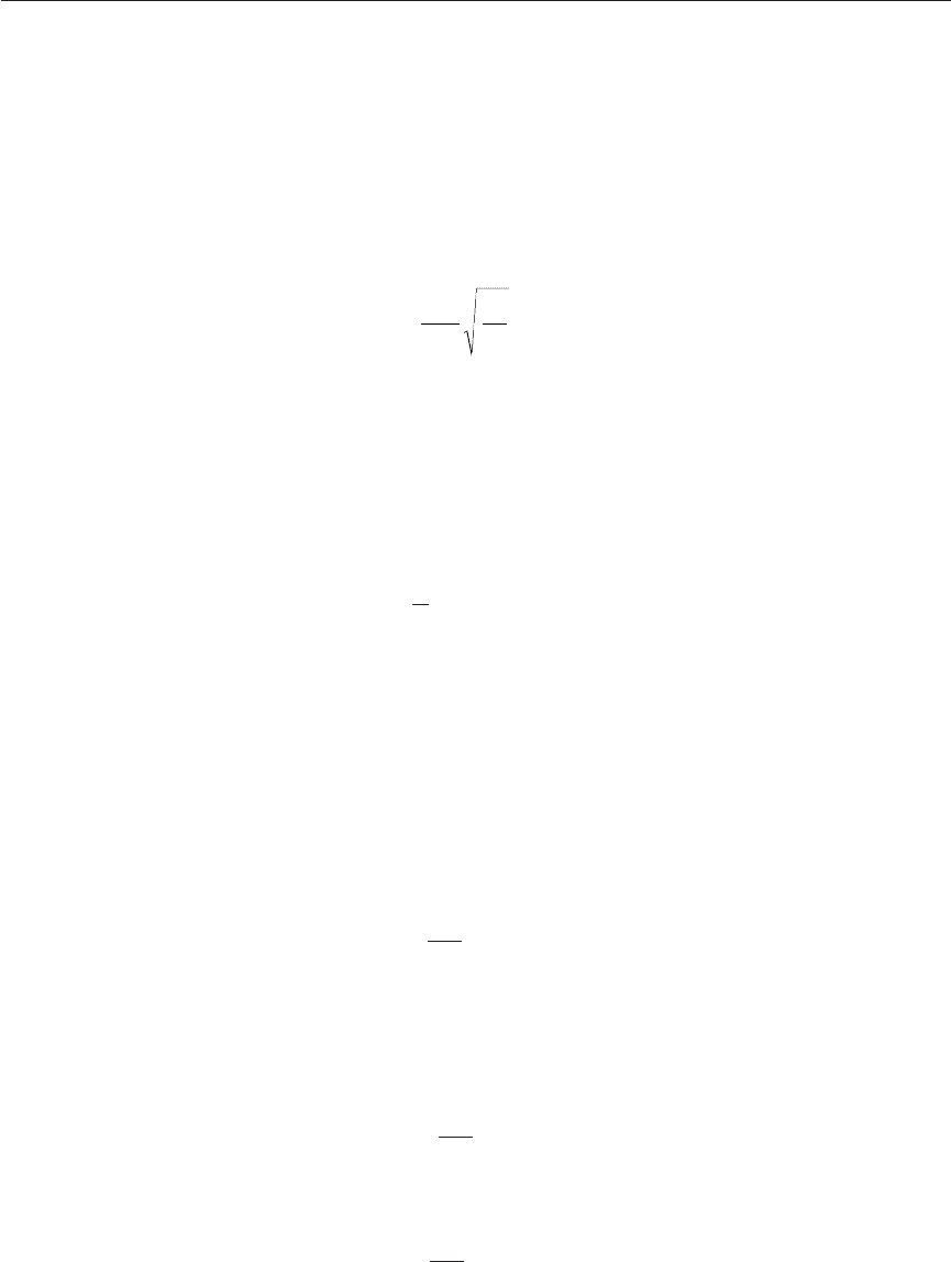
wall shear stress value is obtained from

(9.9)

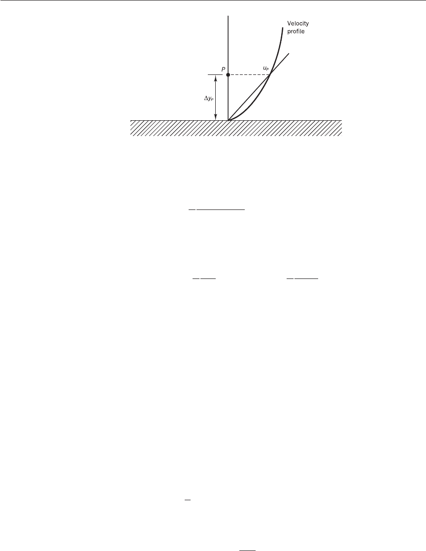
where u

is the velocity at the grid node. Figure 9.13 illustrates that this

formula is based on the assumption that the velocity varies linearly with

distance from the wall in a laminar ﬂow.

The shear force F

is now given by

=−

Cell

=−

Cell

(9.10)

where A

Cell

is the wall area of the control volume. The appropriate source

term in the u-equation is deﬁned by

=− A

Cell

(9.11)

∆y

∆

ANIN_C09.qxd 29/12/2006 10:01 AM Page 275

Heat transfer from a wall at ﬁxed temperature T

into the near-wall cell in

laminar ﬂow is calculated from

=− A

Cell

(9.12)

where C

is the speciﬁc heat of the ﬂuid, T

is the temperature at the node P

and

is the laminar Prandtl number. It is easy to see that the corresponding

source terms for the temperature equation are given by

=− A

Cell

and S

= A

Cell

(9.13)

A ﬁxed heat ﬂux enters the source terms directly by means of the normal

source term linearisation:

= S

+ S

(9.14)

For an adiabatic wall we have, of course, S

= S

= 0.

Turbulent flow

If the value of y

is greater than 11.63 node P is considered to be in the

log-law region of a turbulent boundary layer. In this region wall function

formulae (3.49) and (3.50) associated with the log-law are used to calculate

shear stress, heat ﬂux and other variables. The formulae have been applied

in many different ways but Table 9.1 gives the optimum near-wall relation-

ships from extensive computing trials.

These relationships should be used in conjunction with the universal

velocity and temperature distributions for near-wall turbulent ﬂows in

(3.49)–(3.50):

= ln(Ey

) (3.49)

and

T,t

+ P (3.50)

T,l

T,t

∆y

− T

)

∆y

276 CHAPTER 9 IMPLEMENTATION OF BOUNDARY CONDITIONS

Figure 9.13 Velocity

distribution at a wall

ANIN_C09.qxd 29/12/2006 10:01 AM Page 276