Versteeg H., Malalasekra W. An Introduction to Computational Fluid Dynamics: The Finite Volume Method

Подождите немного. Документ загружается.

2.11 PROBLEMS IN COMPRESSIBLE FLOWS 37

ensure that the limited domain of dependence of effectively inviscid (hyper-

bolic) ﬂows at Mach numbers greater than 1 is adequately modelled. Issa

and Lockwood (1977) and McGuirk and Page (1990) gave lucid papers that

identify the main issues relevant to the ﬁnite volume method.

Open (far ﬁeld) boundary conditions give the most serious problems for

the designer of general-purpose CFD codes. Subsonic inviscid compressible

ﬂow equations require fewer inlet conditions (normally only

and u are spe-

ciﬁed) than viscous ﬂow equations and only one outlet condition (typically

speciﬁed pressure). Supersonic inviscid compressible ﬂows require the same

number of inlet boundary conditions as viscous ﬂows, but do not admit any

outﬂow boundary conditions because the ﬂow is hyperbolic.

Without knowing a great deal about the ﬂow before solving a problem it

is very difﬁcult to specify the precise number and nature of the allowable

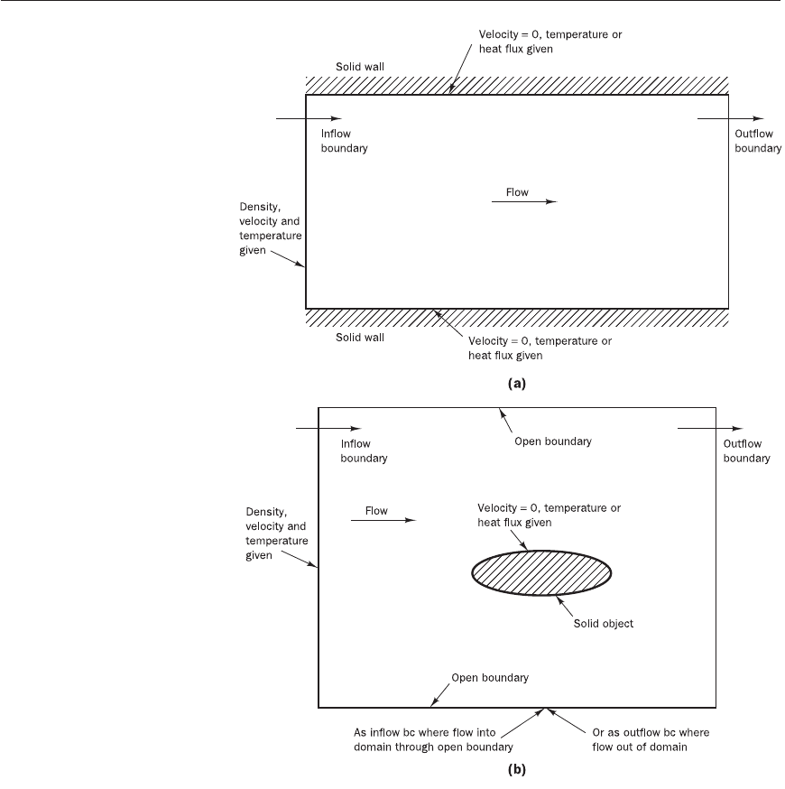
Figure 2.12 (a) Boundary

conditions for an internal ﬂow

problem; (b) boundary condition

for external ﬂow problem

ANIN_C02.qxd 29/12/2006 09:55 AM Page 37

boundary conditions on any ﬂuid/ﬂuid boundary in the far ﬁeld. Issa and

Lockwood’s work (1977) reported the solution of a shock/boundary layer

interaction problem where part of the far ﬁeld boundary conditions are

obtained from an inviscid solution performed prior to the viscous solution.

The usual (viscous) outlet condition

∂

(

∂

n = 0 is applied on the remain-

der of the far ﬁeld boundary.

Fletcher (1991) noted that under-speciﬁcation of boundary conditions

normally leads to failure to obtain a unique solution. Over-speciﬁcation,

however, gives rise to ﬂow solutions with severe and unphysical ‘boundary

layers’ close to the boundary where the condition is applied.

If the location of the outlet or far ﬁeld boundaries is chosen far enough

away from the region of interest within the solution domain it is possible to

get physically meaningful results. Most careful solutions test the sensitivity

of the interior solution to the positioning of outﬂow and far ﬁeld boundaries.

If results do not change in the interior, the boundary conditions are ‘trans-

parent’ and the results are acceptable.

These complexities make it very difﬁcult for general-purpose ﬁnite vol-

ume CFD codes to cope with general subsonic, transonic and/or supersonic

viscous ﬂows. Although all commercially available codes claim to be able to

make computations in all ﬂow regimes, they perform most effectively at

Mach numbers well below 1 as a consequence of all the problems outlined

above.

We have derived the complete set of governing equations of ﬂuid ﬂow from

basic conservation principles. The thermodynamic equilibrium assumption

and the Newtonian model of viscous stresses were enlisted to close the sys-

tem mathematically. Since no particular assumptions were made with regard

to the viscosity, it is straightforward to accommodate a variable viscosity that

is dependent on local conditions. This facilitates the inclusion of ﬂuids with

38 CHAPTER 2 CONSERVATION LAWS OF FLUID MOTION

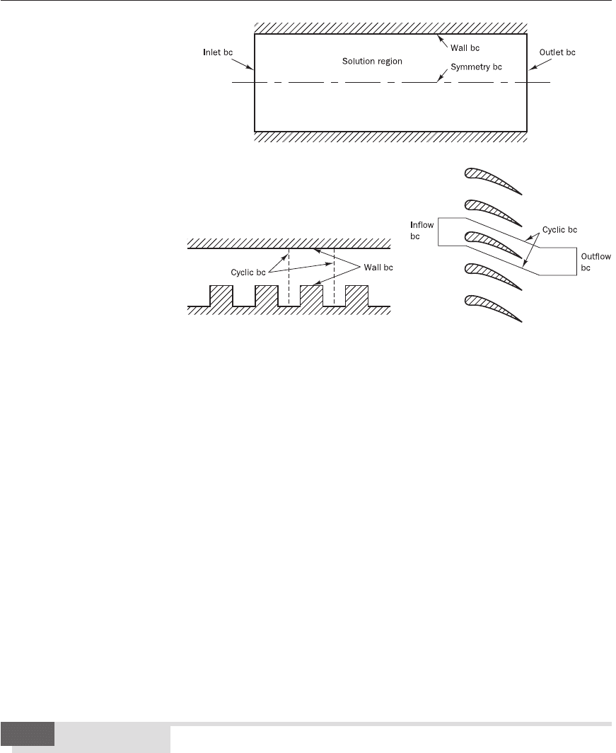
Figure 2.13 Examples of ﬂow

boundaries with symmetry and

cyclic conditions

Summary2.12

ANIN_C02.qxd 29/12/2006 09:55 AM Page 38

2.12 SUMMARY 39

temperature-dependent viscosity and those with non-Newtonian character-

istics within the framework of equations.

We have identiﬁed a common differential form for all the ﬂow equations,

the so-called transport equation, and developed integrated forms which are

central to the ﬁnite volume CFD method:

For steady state processes

n . (

ρφ

u)dA = n . (Γ grad

)dA + S

dV (2.43)

and for time-dependent processes

ρφ

dV dt + n . (

ρφ

u)dA dt

= n . (Γ grad

)dA dt + S

dV dt (2.44)

The auxiliary conditions – initial and boundary conditions – needed to solve

a ﬂuid ﬂow problem were also discussed. It emerged that there are three

types of distinct physical behaviour – elliptic, parabolic and hyperbolic – and

the governing ﬂuid ﬂow equations were formally classiﬁed. Problems with

this formal classiﬁcation were identiﬁed as resulting from: (i) boundary-

layer-type behaviour in ﬂows at high Reynolds numbers and (ii) compress-

ibility effects at Mach numbers around and above 1. These lead to severe

difﬁculties in the speciﬁcation of boundary conditions for completely general-

purpose CFD procedures working at any Reynolds number and Mach

number.

Experience with the ﬁnite volume method has yielded a set of auxiliary

conditions that give physically realistic ﬂow solutions in many industrially

relevant problems. The most complete problem speciﬁcation includes, in

addition to initial values of all ﬂow variables, the following boundary

conditions:

• Complete speciﬁcation of the distribution of all variables

(except

pressure) at all inlets to the ﬂow domain of interest

• Speciﬁcation of pressure at one location inside the ﬂow domain

• Set gradient of all variables

to zero in the ﬂow direction at suitably

positioned outlets

• Speciﬁcation of all variables

(except pressure and density) or their

normal gradients at solid walls



∆t



∆t



∆t



∂



∆t



ANIN_C02.qxd 29/12/2006 09:55 AM Page 39

All ﬂows encountered in engineering practice, simple ones, such as two-

dimensional jets, wakes, pipe ﬂows and ﬂat plate boundary layers, and

more complicated three-dimensional ones, become unstable above a certain

Reynolds number (UL/

where U and L are characteristic velocity and

length scales of the mean ﬂow and

is the kinematic viscosity). At low

Reynolds numbers ﬂows are laminar. At higher Reynolds numbers ﬂows

are observed to become turbulent. A chaotic and random state of motion

develops in which the velocity and pressure change continuously with time

within substantial regions of ﬂow.

Flows in the laminar regime are completely described by the equations

developed in Chapter 2. In simple cases the continuity and Navier–Stokes

equations can be solved analytically (Schlichting, 1979). More complex ﬂows

can be tackled numerically with CFD techniques such as the ﬁnite volume

method without additional approximations.

Many, if not most, ﬂows of engineering signiﬁcance are turbulent, so the

turbulent ﬂow regime is not just of theoretical interest. Fluid engineers need

access to viable tools capable of representing the effects of turbulence. This

chapter gives a brief introduction to the physics of turbulence and to its

modelling in CFD.

In sections 3.1 and 3.2, the nature of turbulent ﬂows and the physics of

the transition from laminar ﬂow to turbulence are examined. In section 3.3

we give formal deﬁnitions for the most common descriptors of a turbulent

ﬂow, and in section 3.4 the characteristics of some simple two-dimensional

turbulent ﬂows are described. Next, in section 3.5, the consequences of

the appearance of the ﬂuctuations associated with turbulence on the time-

averaged Navier–Stokes equations are analysed. The velocity ﬂuctuations

are found to give rise to additional stresses on the ﬂuid, the so-called

Reynolds stresses. The main categories of models for these extra stress terms

are given in section 3.6. The most widely used category of classical turbu-

lence models is discussed in section 3.7. In section 3.8 we review large eddy

simulations (LES) and in section 3.9 we give a brief summary of direct

numerical simulation (DNS).

First we take a brief look at the main characteristics of turbulent ﬂows.

The Reynolds number of a ﬂow gives a measure of the relative importance

of inertia forces (associated with convective effects) and viscous forces.

In experiments on ﬂuid systems it is observed that at values below the so-

called critical Reynolds number Re

crit

the ﬂow is smooth and adjacent layers

Chapter three Turbulence and its modelling

What is

turbulence?

3.1

ANIN_C03.qxd 29/12/2006 04:34PM Page 40

3.1 WHAT IS TURBULENCE? 41

of ﬂuid slide past each other in an orderly fashion. If the applied boundary

conditions do not change with time the ﬂow is steady. This regime is called

laminar ﬂow.

At values of the Reynolds number above Re

crit

a complicated series of

events takes place which eventually leads to a radical change of the ﬂow

character. In the ﬁnal state the ﬂow behaviour is random and chaotic. The

motion becomes intrinsically unsteady even with constant imposed bound-

ary conditions. The velocity and all other ﬂow properties vary in a random

and chaotic way. This regime is called turbulent ﬂow. A typical point velo-

city measurement might exhibit the form shown in Figure 3.1.

Figure 3.1 Typical point

velocity measurement in

turbulent ﬂow

The random nature of a turbulent ﬂow precludes an economical descrip-

tion of the motion of all the ﬂuid particles. Instead the velocity in Figure 3.1

is decomposed into a steady mean value U with a ﬂuctuating component u′(t)

superimposed on it: u(t) = U + u′(t). This is called the Reynolds decom-

position. A turbulent ﬂow can now be characterised in terms of the mean

values of ﬂow properties (U, V, W, P etc.) and some statistical properties of

their ﬂuctuations (u′, v′, w′, p′ etc.). We give formal deﬁnitions of the mean

and the most common statistical descriptors of the ﬂuctuations in section 3.3.

Even in ﬂows where the mean velocities and pressures vary in only

one or two space dimensions, turbulent ﬂuctuations always have a three-

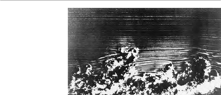
dimensional spatial character. Furthermore, visualisations of turbulent

ﬂows reveal rotational ﬂow structures, so-called turbulent eddies, with a

wide range of length scales. Figure 3.2, which depicts a cross-sectional

view of a turbulent boundary layer on a ﬂat plate, shows eddies whose length

scale is comparable with that of the ﬂow boundaries as well as eddies of inter-

mediate and small size.

Particles of ﬂuid which are initially separated by a long distance can be

brought close together by the eddying motions in turbulent ﬂows. As a

consequence, heat, mass and momentum are very effectively exchanged.

For example, a streak of dye which is introduced at a point in a turbulent

ﬂow will rapidly break up and be dispersed right across the ﬂow. Such

effective mixing gives rise to high values of diffusion coefﬁcients for mass,

momentum and heat.

The largest turbulent eddies interact with and extract energy from the

mean ﬂow by a process called vortex stretching. The presence of mean

velocity gradients in sheared ﬂows distorts the rotational turbulent eddies.

Suitably aligned eddies are stretched because one end is forced to move

faster than the other.

ANIN_C03.qxd 29/12/2006 04:34PM Page 41

The characteristic velocity

and characteristic length  of the larger

eddies are of the same order as the velocity scale U and length scale L of the

mean ﬂow. Hence a ‘large eddy’ Reynolds number Re



/

formed by

combining these eddy scales with the kinematic viscosity will be large in all

turbulent ﬂows, since it is not very different in magnitude from UL/

which itself is large. This suggests that these large eddies are dominated by

inertia effects and viscous effects are negligible.

The large eddies are therefore effectively inviscid, and angular momen-

tum is conserved during vortex stretching. This causes the rotation rate to

increase and the radius of their cross-sections to decrease. Thus the process

creates motions at smaller transverse length scales and also at smaller time

scales. The stretching work done by the mean ﬂow on the large eddies dur-

ing these events provides the energy which maintains the turbulence.

Smaller eddies are themselves stretched strongly by somewhat larger

eddies and more weakly with the mean ﬂow. In this way the kinetic energy is

handed down from large eddies to progressively smaller and smaller eddies

in what is termed the energy cascade. All the ﬂuctuating properties of a

turbulent ﬂow contain energy across a wide range of frequencies or wavenum-

bers (= 2

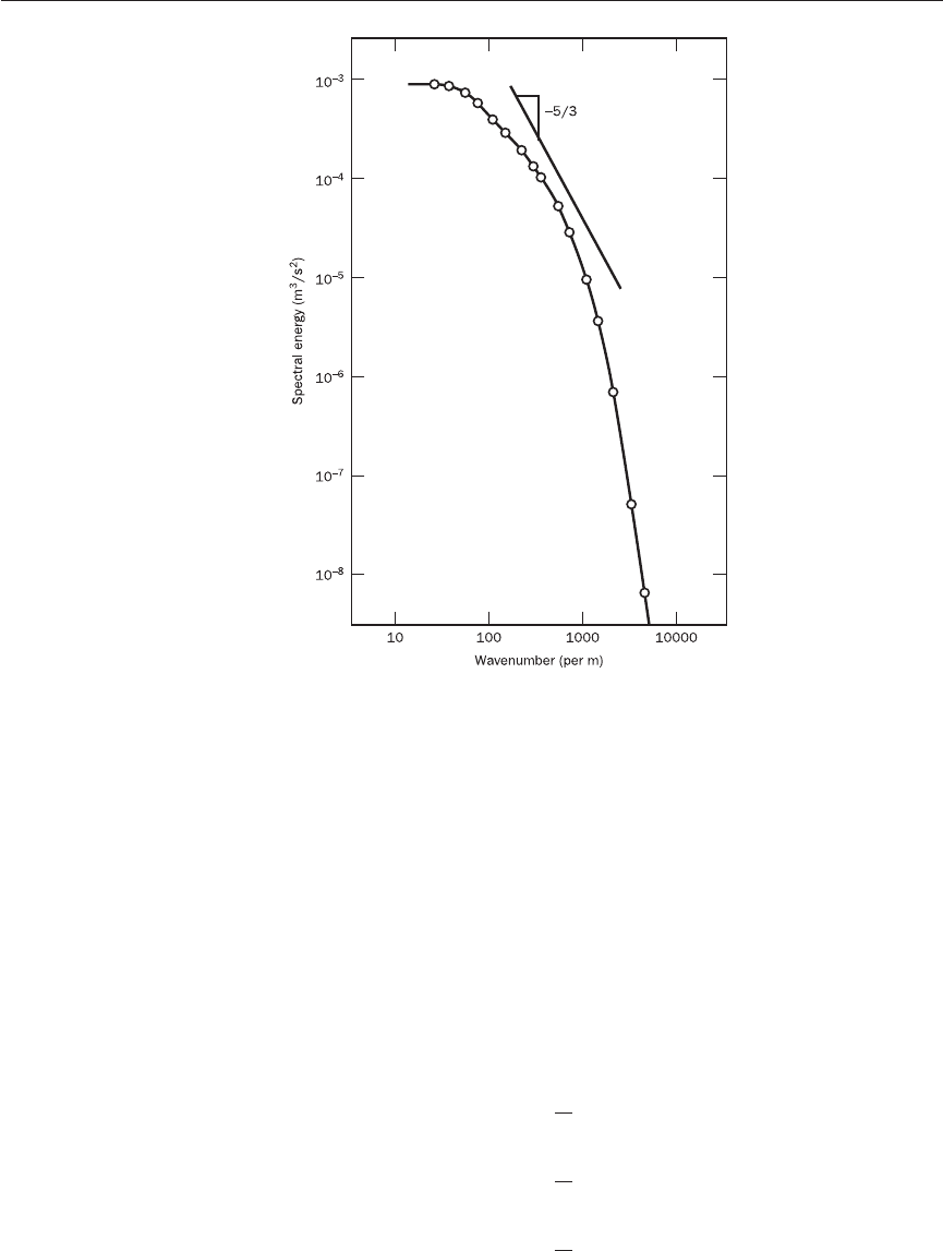
f/U where f is the frequency). This is demonstrated in Figure 3.3,

which gives the energy spectrum of turbulence downstream of a grid.

The spectral energy E(

) is shown as a function of the wavenumber

= 2

, where

is the wavelength of the eddies. The spectral energy E(

)

(units m

) is the kinetic energy per unit mass and per unit wavenumber of

ﬂuctuations around the wavenumber

. The diagram shows that the energy

content peaks at the low wavenumbers, so the larger eddies are the most

energetic. They acquire their energy through strong interactions with the

mean ﬂow. The value of E(

) rapidly decreases as the wavenumber increases,

so the smallest eddies have the lowest energy content.

The smallest scales of motion in a turbulent ﬂow (lengths of the order

of 0.1 to 0.01 mm and frequencies around 10 kHz in typical turbulent

engineering ﬂows) are dominated by viscous effects. The Reynolds number

of the smallest eddies based on their characteristic velocity

and

characteristic length

is equal to 1, Re

υη

= 1, so the smallest scales

present in a turbulent ﬂow are those for which the inertia and viscous effects

42 CHAPTER 3 TURBULENCE AND ITS MODELLING

Figure 3.2 Visualisation of a

turbulent boundary layer

Source: Van Dyke (1982)

ANIN_C03.qxd 29/12/2006 04:34PM Page 42

3.1 WHAT IS TURBULENCE? 43

are of equal strength. These scales are named the Kolmogorov microscales

after the Russian scientist who carried out groundbreaking work on the struc-

ture of turbulence in the 1940s. At these scales work is performed against the

action of viscous stresses, so that the energy associated with small-scale eddy

motions is dissipated and converted into thermal internal energy. This dissipa-

tion results in increased energy losses associated with turbulent ﬂows.

Dimensional analysis can be used to obtain ratios of the length, time and

velocity scales of the small and large eddies. The Kolmogorov microscales

can be expressed in terms of the rate of energy dissipation of a turbulent ﬂow

and the ﬂuid viscosity, which uses the notion that in every turbulent ﬂow the

rate of production of turbulent energy has to be broadly in balance with its

rate of dissipation to prevent unlimited growth of turbulence energy. This

yields the following order of magnitude estimates of the ratios of small

length, time and velocity scales

and large length, time and velocity

scales , T,

(Tennekes and Lumley, 1972; Reynolds in Lumley, 1989):

Length-scale ratio ≈ Re



−3/4

(3.1a)

Time-scale ratio ≈ Re



−1/2

(3.1b)

Velocity-scale ratio ≈ Re



−1/4

(3.1c)



Figure 3.3 Energy spectrum of

turbulence behind a grid

ANIN_C03.qxd 29/12/2006 04:34PM Page 43

Typical values of Re



might be 10

–10

, so the length, time and velocity

scales associated with small dissipating eddies are much smaller than those of

large, energetic eddies, and the difference – the so-called scale separation –

increases as Re



increases.

The behaviour of the large eddies should be independent of viscosity and

should depend on the velocity scale

and length scale . Thus, on dimen-

sional grounds we would expect that the spectral energy content of these

eddies should behave as follows: E(

) ∝

, where

= 1/. Since the length

scale  is related to the length scale of turbulence producing processes – for

example, boundary layer thickness

, obstacle width L, surface roughness

height k

– we expect the structure of the largest eddies to be highly

anisotropic (i.e. the ﬂuctuations are different in different directions) and

strongly affected by the problem boundary conditions.

Kolmogorov argued that the structure of the smallest eddies and, hence,

their spectral energy E(

= 1/

) should only depend on the rate of dissipa-

tion of turbulent energy

(units m

) and the kinematic viscosity of the

ﬂuid

. Dimensional analysis yields the following proportionality relation-

ship for the spectral energy: E(

= 1/

) ∝

5/4

1/4

. Thus, the spectral energy

) of the smallest eddies only depends on the problem through the rate of

energy dissipation and is not linked to other problem variables. The diffusive

action of viscosity tends to smear out directionality at small scales. At high

mean ﬂow Reynolds numbers the smallest eddies in a turbulent ﬂow are,

therefore, isotropic (non-directional).

Finally, Kolmogorov derived the universal spectral properties of eddies of

intermediate size, which are sufﬁciently large for their behaviour to be un-

affected by viscous action (as the larger eddies), but sufﬁciently small that the

details of their behaviour can be expressed as a function of the rate of energy

dissipation

(as the smallest eddies). The appropriate length scale for these

eddies is 1/

, and he found that the spectral energy of these eddies – the

inertial subrange – satisﬁes the following relationship: E(

) =

ακ

−5/3

2/3

Measurements showed that the constant

≈ 1.5. Figure 3.3 includes a line

with a slope of −5/3, indicating that, for the measurements shown, the scale

separation is insufﬁcient for a clear inertial subrange. Overlap between the

large and small eddies is located somewhere around

≈ 1000.

The initial cause of the transition to turbulence can be explained by con-

sidering the stability of laminar ﬂows to small disturbances. A sizeable body

of theoretical work is devoted to the analysis of the inception of transition:

hydrodynamic instability. In many relevant instances the transition to

turbulence is associated with sheared ﬂows. Linear hydrodynamic stability

theory seeks to identify conditions which give rise to ampliﬁcation of disturb-

ances. Of particular interest in an engineering context is the prediction of the

values of the Reynolds numbers Re

x,crit

(= Ux

crit

) at which disturbances are

ampliﬁed and Re

x,tr

(= Ux

) at which transition to fully turbulent ﬂow

takes place.

A mathematical discussion of the theory is beyond the scope of this brief

introduction. White (1991) gave a useful overview of theory and experi-

ments. The subject matter is fairly complex but its conﬁrmation has led to a

series of experiments which reveal the physical processes causing transition

from laminar to turbulent ﬂow. Most of our knowledge stems from work on

44 CHAPTER 3 TURBULENCE AND ITS MODELLING

Transition from

laminar to

turbulent flow

3.2

ANIN_C03.qxd 29/12/2006 04:34PM Page 44

3.2 TRANSITION FROM LAMINAR TO TURBULENT FLOW 45

two-dimensional incompressible ﬂows. All such ﬂows are sensitive to two-

dimensional disturbances with a relatively long wavelength, several times the

transverse distance over which velocity changes take place (e.g. six times the

thickness of a ﬂat plate boundary layer).

Hydrodynamic stability of laminar flows

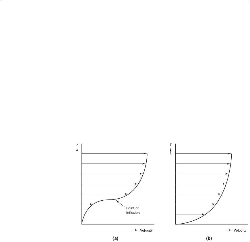
Two fundamentally different instability mechanisms operate, which are

associated with the shape of the two-dimensional laminar velocity proﬁle

of the base ﬂow. Flows with a velocity distribution which contains a point

of inﬂexion as shown in Figure 3.4a are always unstable with respect to

inﬁnitesimal disturbances if the Reynolds number is large enough. This

instability was ﬁrst identiﬁed by making an inviscid assumption in the equa-

tions describing the evolution of the disturbances. Subsequent reﬁnement

of the theory by inclusion of the effect of viscosity changed its results very

little, so this type of instability is known as inviscid instability. Velocity

proﬁles of the type shown in Figure 3.4a are associated with jet ﬂows, mix-

ing layers and wakes and also with boundary layers over ﬂat plates under the

inﬂuence of an adverse pressure gradient (

∂

x > 0). The role of viscosity

is to dampen out ﬂuctuations and stabilise the ﬂow at low Reynolds numbers.

Figure 3.4 Velocity proﬁles

susceptible to (a) inviscid

instability and (b) viscous

instability

Flows with laminar velocity distributions without a point of inﬂexion such

as the proﬁle shown in Figure 3.4b are susceptible to viscous instability.

The approximate inviscid theory predicts unconditional stability for these

velocity proﬁles, which are invariably associated with ﬂows near solid walls

such as pipe, channel and boundary layer ﬂows without adverse pressure

gradients (

∂

x ≤ 0). Viscous effects play a more complex role providing

damping at low and high Reynolds numbers, but contributing to the destabil-

isation of the ﬂows at intermediate Reynolds numbers.

Transition to turbulence

The point where instability ﬁrst occurs is always upstream of the point of

transition to fully turbulent ﬂow. The distance between the point of instab-

ility where the Reynolds number equals Re

x,crit

and the point of transition

ANIN_C03.qxd 29/12/2006 04:34PM Page 45

x,tr

depends on the degree of ampliﬁcation of the unstable disturbances.

The point of instability and the onset of the transition process can be pre-

dicted with the linear theory of hydrodynamic instability. There is, however,

no comprehensive theory regarding the path leading from initial instability

to fully turbulent ﬂows. Next, we describe the main, experimentally observed,

characteristics of three simple ﬂows: jets, ﬂat plate boundary layers and pipe

ﬂows.

Jet flow: an example of a flow with a point of inflexion

Flows which possess one or more points of inﬂexion amplify long-

wavelength disturbances at all Reynolds numbers typically above about 10.

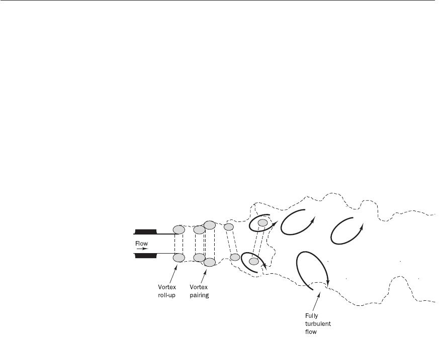
The transition process is explained by considering the sketch of a jet ﬂow

(Figure 3.5).

46 CHAPTER 3 TURBULENCE AND ITS MODELLING

Figure 3.5 Transition in

a jet ﬂow

After the ﬂow emerges from the oriﬁce the laminar exit ﬂow produces the

rolling up of a vortex fairly close to the oriﬁce. Subsequent ampliﬁcation

involves the formation of a single vortex of greater strength through the pair-

ing of vortices. A short distance further downstream, three-dimensional dis-

turbances cause the vortices to become heavily distorted and less distinct.

The ﬂow breaks down, generating a large number of small-scale eddies, and

the ﬂow undergoes rapid transition to the fully turbulent regime. Mixing

layers and wakes behind bluff bodies exhibit a similar sequence of events,

leading to transition and turbulent ﬂow.

Boundary layer on a flat plate: an example of a flow without a

point of inflexion

In ﬂows with a velocity distribution without a point of inﬂexion viscous

instability theory predicts that there is a ﬁnite region of Reynolds numbers

around Re

= 1000 (

is the boundary layer thickness) where inﬁnitesimal

disturbances are ampliﬁed. The developing ﬂow over a ﬂat plate is such a

ﬂow, and the transition process has been extensively researched for this case.

The precise sequence of events is sensitive to the level of disturbance of

the incoming ﬂow. However, if the ﬂow system creates sufﬁciently smooth con-

ditions the instability of a boundary layer ﬂow to relatively long-wavelength

ANIN_C03.qxd 29/12/2006 04:34PM Page 46