Versteeg H., Malalasekra W. An Introduction to Computational Fluid Dynamics: The Finite Volume Method

Подождите немного. Документ загружается.

3.2 TRANSITION FROM LAMINAR TO TURBULENT FLOW 47

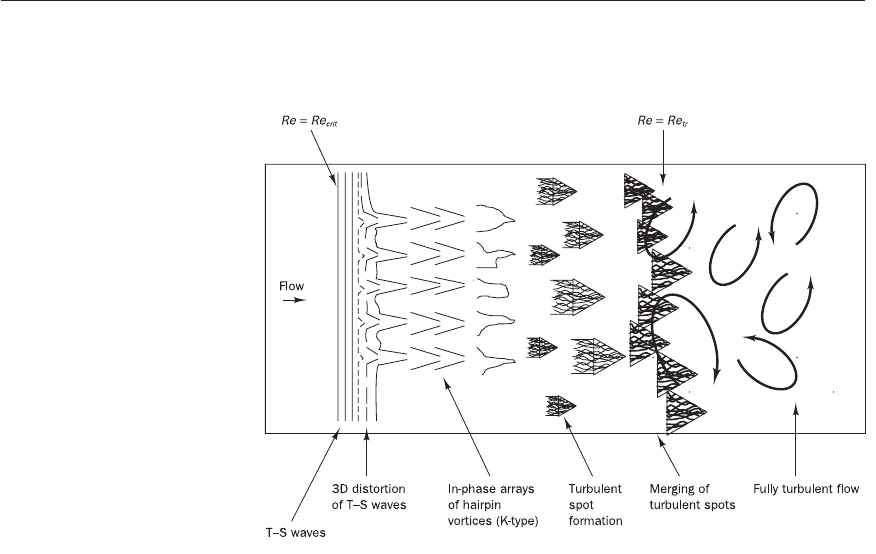
disturbances can be clearly detected. A sketch of the processes leading to

transition and fully turbulent ﬂow is given in Figure 3.6.

Figure 3.6 Plan view sketch of

transition processes in boundary

layer ﬂow over a ﬂat plate

If the incoming ﬂow is laminar numerous experiments conﬁrm the

predictions of the theory that initial linear instability occurs around Re

x,crit

91 000. The unstable two-dimensional disturbances are called Tollmien–

Schlichting (T–S) waves. These disturbances are ampliﬁed in the ﬂow

direction.

The subsequent development depends on the amplitude of the waves

at maximum (linear) ampliﬁcation. Since ampliﬁcation takes place over a

limited range of Reynolds numbers, it is possible that the ampliﬁed waves

are attenuated further downstream and that the ﬂow remains laminar. If the

amplitude is large enough a secondary, non-linear, instability mechanism

causes the Tollmien–Schlichting waves to become three-dimensional and

ﬁnally evolve into hairpin Λ-vortices. In the most common mechanism of

transition, so-called K-type transition, the hairpin vortices are aligned.

Above the hairpin vortices a high shear region is induced which subse-

quently intensiﬁes, elongates and rolls up. Further stages of the transition

process involve a cascading breakdown of the high shear layer into smaller

units with frequency spectra of measurable ﬂow parameters approaching

randomness. Regions of intense and highly localised changes occur at random

times and locations near the solid wall. Triangular turbulent spots burst from

these locations. These turbulent spots are carried along with the ﬂow and

grow by spreading sideways, which causes increasing amounts of laminar

ﬂuid to take part in the turbulent motion.

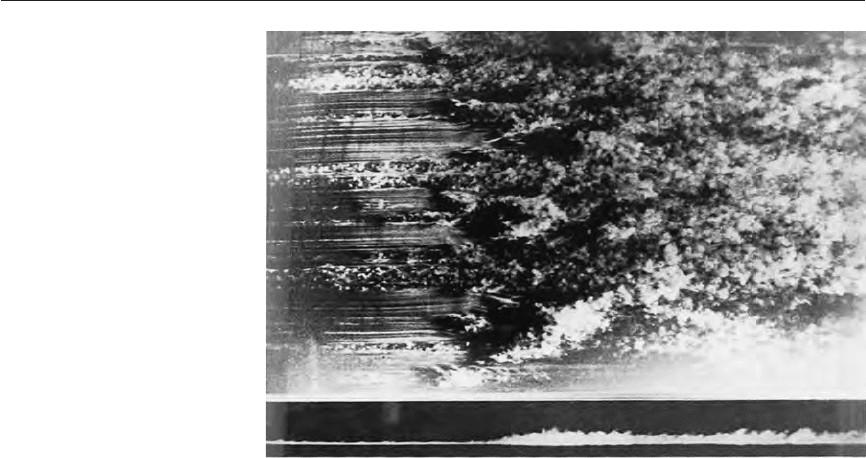
Transition of a natural ﬂat plate boundary layer involves the formation

of turbulent spots at active sites and the subsequent merging of different tur-

bulent spots convected downstream by the ﬂow. This takes place at Reynolds

numbers Re

x,tr

≈ 10

. Figure 3.7 is a plan view snapshot of a ﬂat plate boundary

layer that illustrates this process.

ANIN_C03.qxd 29/12/2006 04:34PM Page 47

Pipe flow transition

The transition in a pipe ﬂow represents an example of a special category

of ﬂows without an inﬂexion point. The viscous theory of hydrodynamic

stability predicts that these ﬂows are unconditionally stable to inﬁnitesimal

disturbances at all Reynolds numbers. In practice, transition to turbulence

takes place between Re (= UD/

) 2000 and 10

. Various details are still

unclear, which illustrates the limitations of current stability theories.

The cause of the apparent failure of the theory is almost certainly the

role played by distortions of the inlet velocity proﬁle and the ﬁnite amplitude

disturbances due to entry effects. Experiments show that in pipe ﬂows, as

in ﬂat plate boundary layers, turbulent spots appear in the near-wall region.

These grow, merge and subsequently ﬁll the pipe cross-section to form tur-

bulent slugs. In industrial pipe ﬂows intermittent formation of turbulent

slugs takes place at Reynolds numbers around 2000 giving rise to alternate

turbulent and laminar regions along the length of the pipe. At Reynolds

numbers above 2300 the turbulent slugs link up and the entire pipe is ﬁlled

with turbulent ﬂow.

Final comments

It is clear from the above descriptions of transition in jets, ﬂat plate bound-

ary layers and pipe ﬂows that there are a number of common features in

the transition processes: (i) the ampliﬁcation of initially small disturbances,

(ii) the development of areas with concentrated rotational structures, (iii) the

formation of intense small-scale motions and ﬁnally (iv) the growth and

merging of these areas of small-scale motions into fully turbulent ﬂows.

The transition to turbulence is strongly affected by factors such as

pressure gradient, disturbance levels, wall roughness and heat transfer. The

discussions only apply to subsonic, incompressible ﬂows. The appearance of

48 CHAPTER 3 TURBULENCE AND ITS MODELLING

Figure 3.7 Merging of

turbulent spots and transition

to turbulence in a ﬂat plate

boundary layer

Source: Nakayama (1988)

ANIN_C03.qxd 29/12/2006 04:34PM Page 48

3.3 DESCRIPTORS OF TURBULENT FLOW 49

signiﬁcant compressibility effects in ﬂows at Mach numbers above about 0.7

greatly complicates the stability theory.

It should be noted that although a great deal has been learnt from simple

ﬂows, there is no comprehensive theory of transition. Advances in super-

computer technology have made it possible to simulate the events leading up

to transition, including turbulent spot formation, and turbulence at modest

Reynolds numbers by solving the complete, time-dependent Navier–Stokes

equations for simple geometries. Kleiser and Zang (1991) gave a review

which highlights very favourable agreement between experiments and their

computations.

For engineering purposes the major case where the transition process

inﬂuences a sizeable fraction of the ﬂow is that of external wall boundary

layer ﬂows at intermediate Reynolds numbers. This occurs in certain turbo-

machines, helicopter rotors and some low-speed aircraft wings. Cebeci

(1989) presented an engineering calculation method based on a combination

of inviscid far ﬁeld and boundary layer computations in conjunction with

a linear stability analysis to identify the critical and transition Reynolds num-

bers. Transition is deemed to have occurred at the point where an (arbitrary)

ampliﬁcation factor e

(≈ 8000) of initial disturbances is found. The proced-

ure, which includes a mixing length model (see section 3.6.1) for the fully

turbulent part of the boundary layer, has proved very effective for aerofoil

calculations, but requires a substantial amount of empirical input and there-

fore lacks generality.

Commercially available general-purpose CFD procedures often ignore

transition entirely and classify ﬂows as either laminar or fully turbulent. The

transition region often constitutes only a very small fraction of the size of the

ﬂow domain and in those cases it is assumed that the errors made by neglect-

ing its detailed structure are only small.

Let us consider a single point measurement in a turbulent ﬂow, e.g. a velo-

city measurement made with a hot-wire anemometer (Comte-Bellot, 1976)

or a laser Doppler anemometer (Buchhave et al., 1979) or a local pressure

measurement made with a small transducer. In Figure 3.1, we saw that the

appearance of turbulence manifested itself as random ﬂuctuations of the

measured velocity component about a mean value. All other ﬂow variables,

i.e. all other velocity components, the pressure, temperature, density etc.,

will also exhibit this additional time-dependent behaviour. The Reynolds

decomposition deﬁnes ﬂow property

at this point as the sum of a steady

mean component Φ and a time varying ﬂuctuating component

′(t) with zero

mean value: hence

(t) =Φ+

′(t). We start with a formal deﬁnition of the

time average or mean Φ and we also deﬁne the most widely used statistical

descriptors of the ﬂuctuating component

′.

Time average or mean

The mean Φ of ﬂow property

is deﬁned as follows:

Φ=

(t)dt (3.2)

∆t



∆t

Descriptors of

turbulent flow

3.3

ANIN_C03.qxd 29/12/2006 04:34PM Page 49

In theory we should take the limit of time interval ∆t approaching inﬁnity,

but the process indicated by equation (3.2) gives meaningful time averages

if ∆t is larger than the time scale associated with the slowest variations (due

to the largest eddies) of property

. This deﬁnition of the mean of a ﬂow

property is adequate for steady mean ﬂows. In time-dependent ﬂows the

mean of a property at time t is taken to be the average of the instantaneous

values of the property over a large number of repeated identical experiments:

the so-called ‘ensemble average’.

The time average of the ﬂuctuations

′ is, by deﬁnition, zero:

′(t) dt ≡ 0 (3.3)

From now on we shall not write down the time-dependence of

and

′

explicitly, so we write

=Φ+

′.

The most compact description of the main characteristics of the ﬂuctuat-

ing component of a turbulent ﬂow variable is in terms of its statistics.

Variance, r.m.s. and turbulence kinetic energy

The descriptors used to indicate the spread of the ﬂuctuations

′ about the

mean value Φ are the variance and root mean square (r.m.s.):

= (

′)

dt (3.4a)

rms

==(

′)

1/2

(3.4b)

The r.m.s. values of the velocity components are of particular importance

since they are generally most easily measured and express the average

magnitude of velocity ﬂuctuations. In section 3.5 we will come across the

variances of velocity ﬂuctuations , and when we consider the time

average of the Navier–Stokes equations and ﬁnd that they are proportional

to the momentum ﬂuxes induced by turbulent eddies, which cause additional

normal stresses experienced by ﬂuid elements in a turbulent ﬂow.

One-half times these variances has a further interpretation as the mean

kinetic energy per unit mass contained in the respective velocity ﬂuctuations.

The total kinetic energy per unit mass k of the turbulence at a given location

can be found as follows:

k =++ (3.5)

The turbulence intensity T

is the average r.m.s. velocity divided by a refer-

ence mean ﬂow velocity U

ref

and is linked to the turbulence kinetic energy k

as follows:

= (3.6)

(

–

1/2

ref

w′

v′

u′

w′

v′

u′

∆t



∆t

(

′)

∆t



∆t

(

′)

∆t



∆t

′

50 CHAPTER 3 TURBULENCE AND ITS MODELLING

ANIN_C03.qxd 29/12/2006 04:34PM Page 50

3.3 DESCRIPTORS OF TURBULENT FLOW 51

Moments of different fluctuating variables

The variance is also called the second moment of the ﬂuctuations. Important

details of the structure of the ﬂuctuations are contained in moments constructed

from pairs of different variables. For example, consider properties

=Φ+

′

and

=Ψ+

′ with ==0. Their second moment is deﬁned as

′

′dt (3.7)

If velocity ﬂuctuations in different directions were independent random

ﬂuctuations, then the values of the second moments of the velocity compon-

ents , and would be equal to zero. However, as we have seen,

turbulence is associated with the appearance of vortical ﬂow structures and

the induced velocity components are chaotic, but not independent, so in turn

the second moments are non-zero. In section 3.5 we will come across ,

and again in the time-average of the Navier–Stokes equations.

They represent turbulent momentum ﬂuxes that are closely linked with the

additional shear stresses experienced by ﬂuid elements in turbulent ﬂows.

Pressure–velocity moments, , etc., play a role in the diffusion of

turbulent energy.

Higher-order moments

Additional information relating to the distribution of the ﬂuctuations can be

obtained from higher-order moments. In particular, the third and fourth

moments are related to the skewness (asymmetry) and kurtosis (peakedness),

respectively:

= (

′)

dt (3.8)

= (

′)

dt (3.9)

Correlation functions --- time and space

More detailed information relating to the structure of the ﬂuctuations can be

obtained by studying the relationship between the ﬂuctuations at different

times. The autocorrelation function R

′

(

) is deﬁned as

′

(

) ==

′(t)

′(t +

)dt (3.10)

Similarly, it is possible to deﬁne a further autocorrelation function R

′

(

)

based on two measurements shifted by a certain distance in space:

′

(

) ==

′(x,t′)

′(x +

,t′)dt′ (3.11)

t+∆t



∆t

′(x,t)

′(x +

,t)

∆t



∆t

′(t)

′(t +

)

∆t



∆t

(

′)

∆t



∆t

(

′)

p′v′p′u′

v′w′u′w′

u′v′

v′w′u′w′u′v′

∆t



∆t

′

ANIN_C03.qxd 29/12/2006 04:34PM Page 51

When time shift

(or displacement

) is zero the value of the autocorrelation

function R

′

(0) (or R

′

(0)) just corresponds to the variance and will

have its largest possible value, because the two contributions are perfectly

correlated. Since the behaviour of the ﬂuctuations

′ is chaotic in a turbulent

ﬂow, we expect that the ﬂuctuations become increasingly decorrelated as

→∞(or |

|→∞), so values of the time or space autocorrelation functions

will decrease to zero. The eddies at the root of turbulence cause a certain

degree of local structure in the ﬂow, so there will be correlation between the

values of

′ at time t and a short time later or at a given location x and a small

distance away. The decorrelation process will take place gradually over the

lifetime (or size scale) of a typical eddy. The integral time and length scale,

which represent concrete measures of the average period or size of a turbu-

lent eddy, can be computed from integrals of the autocorrelation function

′

(

) with respect to time shift

or R

′

(

) with respect to distance in the

direction of one of the components of displacement vector

By analogy it is also possible to deﬁne cross-correlation functions

′

(

) with respect to time shift

or R

′

(

) between pairs of different

ﬂuctuations by replacing the second

′ by

′ in equations (3.10) and (3.11).

Probability density function

Finally, we mention the probability density function P(

*), which is

related to the fraction of time that a ﬂuctuating signal spends between

and

* + d

. This is deﬁned in terms of a probability as follows:

*)d

* = Prob(

* <

* + d

*) (3.12)

The average, variance and higher moments of the variable and its ﬂuctu-

ations are related to the probability density function as follows:

(3.13a)

= (

′)

′)d

′ (3.13b)

In equation (3.13b) we can use n = 2 to obtain the variance of

′ and n = 3, 4

. . . for higher-order moments. Probability density functions are used exten-

sively in the modelling of combustion and we come across them again in

Chapter 12.

Most of the theory of turbulent ﬂow was initially developed by careful exam-

ination of the turbulence structure of thin shear layers. In such ﬂows large

velocity changes are concentrated in thin regions. Expressed more formally,

the rates of change of ﬂow variables in the (x-)direction of the ﬂow are negli-

gible compared with the rates of change in the cross-stream (y-)direction

(

∂ϕ

∂

x 

∂ϕ

∂

y). Furthermore, the cross-stream width

of the region over

which changes take place is always small compared with any length scale L

in the ﬂow direction (

/L  1). In the context of this brief introduction we

review the characteristics of some simple two-dimensional incompressible

∞



−∞

(

′)

∞



−∞

′

52 CHAPTER 3 TURBULENCE AND ITS MODELLING

Characteristics

of simple

turbulent flows

3.4

ANIN_C03.qxd 29/12/2006 04:34PM Page 52

3.4 CHARACTERISTICS OF SIMPLE TURBULENT FLOWS 53

turbulent ﬂows with constant imposed pressure. The following ﬂows will be

considered here:

Free turbulent ﬂows

• mixing layer

• jet

• wake

Boundary layers near solid walls

• ﬂat plate boundary layer

• pipe ﬂow

We review data for the mean velocity distribution U = U(y) and the pertinent

second moments , , and .

3.4.1 Free turbulent flows

Among the simplest ﬂows of signiﬁcant engineering importance are those in

the category of free turbulent ﬂows: mixing layers, jets and wakes. A mixing

layer forms at the interface of two regions: one with fast and the other with

slow moving ﬂuid. In a jet a region of high-speed ﬂow is completely sur-

rounded by stationary ﬂuid. A wake is formed behind an object in a ﬂow, so

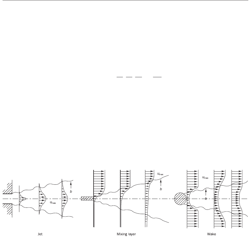
here a slow moving region is surrounded by fast moving ﬂuid. Figure 3.8 is

a sketch of the development of the mean velocity distribution in the stream-

wise direction for these free turbulent ﬂows.

u′v′w′

v′

u′

Figure 3.8 Free turbulent ﬂows

It is clear that velocity changes across an initially thin layer are important

in all three ﬂows. Transition to turbulence occurs after a very short distance

in the ﬂow direction from the point where the different streams initially

meet; the turbulence causes vigorous mixing of adjacent ﬂuid layers and

rapid widening of the region across which the velocity changes take place.

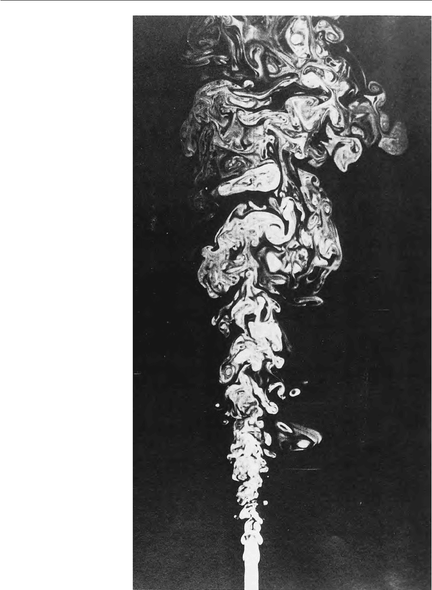
Figure 3.9 shows a visualisation of a jet ﬂow. It is immediately clear that

the turbulent part of the ﬂow contains a wide range of length scales. Large

eddies with a size comparable to the width across the ﬂow are occurring

alongside eddies of very small size.

The visualisation correctly suggests that the ﬂow inside the jet region is

fully turbulent, but the ﬂow in the outer region far away from the jet is

smooth and largely unaffected by the turbulence. The position of the edge of

the turbulent zone is determined by the (time-dependent) passage of indi-

vidual large eddies. Close to the edge these will occasionally penetrate into

ANIN_C03.qxd 29/12/2006 04:34PM Page 53

54 CHAPTER 3 TURBULENCE AND ITS MODELLING

Figure 3.9 Visualisation of a jet

ﬂow

Source: Van Dyke (1982)

ANIN_C03.qxd 29/12/2006 04:34PM Page 54

3.4 CHARACTERISTICS OF SIMPLE TURBULENT FLOWS 55

the surrounding region. During the resulting bursts of turbulent activity in

the outer region – called intermittency – ﬂuid from the surroundings is

drawn into the turbulent zone. This process is termed entrainment and is

the main cause of the spreading of turbulent ﬂows (including wall boundary

layers) in the ﬂow direction.

Initially fast moving jet ﬂuid will lose momentum to speed up the sta-

tionary surrounding ﬂuid. Due to the entrainment of surrounding ﬂuid the

velocity gradients decrease in magnitude in the ﬂow direction. This causes

the decrease of the mean speed of the jet at its centreline. Similarly the dif-

ference between the speed of the wake ﬂuid and its fast moving surroundings

will decrease in the ﬂow direction. In mixing layers the width of the layer

containing the velocity change continues to increase in the ﬂow direction but

the overall velocity difference between the two outer regions is unaltered.

Experimental observations of many such turbulent ﬂows show that after

a certain distance their structure becomes independent of the exact nature of

the ﬂow source. Only the local environment appears to control the turbu-

lence in the ﬂow. The appropriate length scale is the cross-stream layer

width (or half width) b. We ﬁnd that if y is the distance in the cross-stream

direction

= f = g = h (3.14)

for mixing layers for jets for wakes

In these formulae U

max

and U

min

represent the maximum and minimum

mean velocity at a distance x downstream of the source (see Figure 3.8).

Hence, if these local mean velocity scales are chosen and x is large enough,

the functions f, g and h are independent of distance x in the ﬂow direction.

Such ﬂows are called self-preserving.

The turbulence structure also reaches a self-preserving state, albeit after

a greater distance from the ﬂow source than the mean velocity. Then

= f

(3.15)

The velocity scale U

ref

is, as above, (U

max

− U

min

) for a mixing layer and wakes

and U

max

for jets. The precise form of functions f, g, h and f

varies from ﬂow

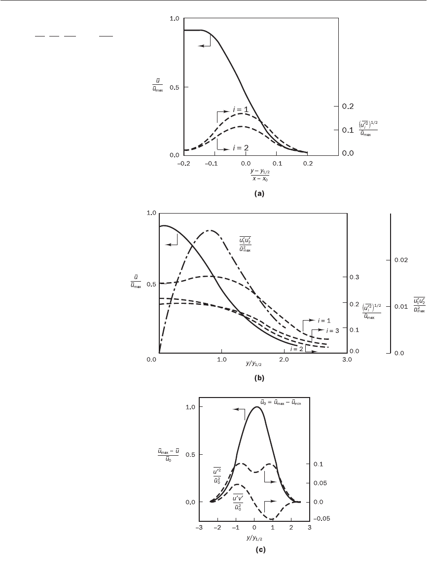
to ﬂow. Figure 3.10 gives mean velocity and turbulence data for a mixing

layer (Champagne et al., 1976), a jet (Gutmark and Wygnanski, 1976) and a

wake ﬂow (Wygnanski et al., 1986).

The largest values of , , and − are found in the region where

the mean velocity gradient

∂

y is largest, highlighting the intimate con-

nection between turbulence production and sheared mean ﬂows. In the ﬂows

shown above the component u′ gives the largest of the normal stresses; its

r.m.s. value has a maximum of 15–40% of the local maximum mean ﬂow

velocity. The fact that the ﬂuctuating velocities are not equal implies an

anisotropic structure of the turbulence.

As |y/b | increases above unity the mean velocity gradients and the veloc-

ity ﬂuctuations all tend to zero. It should also be noted that the turbulence

u′v′w′

v′

u′

u′v′

ref

w′

ref

v′

ref

u′

ref

max

− U

max

− U

min

max

U − U

min

max

− U

min

ANIN_C03.qxd 29/12/2006 04:34PM Page 55

56 CHAPTER 3 TURBULENCE AND ITS MODELLING

Figure 3.10 Distribution of

mean velocity and second

moments , , and −

for incompressible mixing layer,

jet and wake

u′v′w′

v′

u′

ANIN_C03.qxd 29/12/2006 04:34PM Page 56