Versteeg H., Malalasekra W. An Introduction to Computational Fluid Dynamics: The Finite Volume Method

Подождите немного. Документ загружается.

3.4 CHARACTERISTICS OF SIMPLE TURBULENT FLOWS 57

properties become more isotropic. The absence of shear means that turbu-

lence cannot be sustained in this region.

The mean velocity gradient is also zero at the centreline of jets and wakes

and hence no turbulence is produced here. Nevertheless, the values of ,

and do not decrease very much because vigorous eddy mixing trans-

ports turbulent ﬂuid from nearby regions of high turbulence production

towards and across the centreline. The value of − has to become zero

at the centreline of jet and wake ﬂows since it must change sign here by

symmetry.

3.4.2 Flat plate boundary layer and pipe flow

Next we will examine the characteristics of two turbulent ﬂows near solid

walls. Due to the presence of the solid boundary, the ﬂow behaviour and

turbulence structure are considerably different from free turbulent ﬂows.

Dimensional analysis has greatly assisted in correlating the experimental

data. In turbulent thin shear layer ﬂows a Reynolds number based on a

length scale L in the ﬂow direction (or pipe radius) Re

is always very large

(e.g. U = 1 m/s, L = 0.1 m and

= 10

−6

/s gives Re

= 10

). This implies

that the inertia forces are overwhelmingly larger than the viscous forces at

these scales.

If we form a Reynolds number based on a distance y away from the wall

(Re

= Uy/

) we see that if the value of y is of the order of L the above

argument holds. Inertia forces dominate in the ﬂow far away from the wall.

As y is decreased to zero, however, a Reynolds number based on y will also

decrease to zero. Just before y reaches zero there will be a range of values of

y for which Re

is of the order of 1. At this distance from the wall and closer

the viscous forces will be equal in order of magnitude to inertia forces

or larger. To sum up, in ﬂows along solid boundaries there is usually a

substantial region of inertia-dominated ﬂow far away from the wall and a thin

layer within which viscous effects are important.

Close to the wall the ﬂow is inﬂuenced by viscous effects and does not

depend on free stream parameters. The mean ﬂow velocity only depends on

the distance y from the wall, ﬂuid density

and viscosity

and the wall shear

stress

. So

U = f ( y,

)

Dimensional analysis shows that

==f = f (y

) (3.16)

Formula (3.16) is called the law of the wall and contains the deﬁnitions of

two important dimensionless groups, u

and y

. Note that the appropriate

velocity scale is u

, the so-called friction velocity.

Far away from the wall we expect the velocity at a point to be inﬂuenced

by the retarding effect of the wall through the value of the wall shear stress,

but not by the viscosity itself. The length scale appropriate to this region is

the boundary layer thickness

. In this region we have

U = g(y,

)

u′v′

w′

v′

u′

ANIN_C03.qxd 29/12/2006 04:34PM Page 57

58 CHAPTER 3 TURBULENCE AND ITS MODELLING

Dimensional analysis yields

==g

The most useful form emerges if we view the wall shear stress as the cause

of a velocity deﬁcit U

max

− U which decreases the closer we get to the edge

of the boundary layer or the pipe centreline. Thus

= g (3.17)

This formula is called the velocity-defect law.

Linear or viscous sub-layer --- the fluid layer in contact with a

smooth wall

At the solid surface the ﬂuid is stationary. Turbulent eddying motions must also

stop very close to the wall and the behaviour of the ﬂuid closest to the wall is

dominated by viscous effects. This viscous sub-layer is in practice extremely

thin ( y

< 5) and we may assume that the shear stress is approximately con-

stant and equal to the wall shear stress

throughout the layer. Thus

( y) =

≅

After integration with respect to y and application of boundary condition

U = 0 if y = 0, we obtain a linear relationship between the mean velocity and

the distance from the wall

U =

After some simple algebra and making use of the deﬁnitions of u

and y

this

leads to

= y

(3.18)

Because of the linear relationship between velocity and distance from the wall

the ﬂuid layer adjacent to the wall is also known as the linear sub-layer.

Log-law layer --- the turbulent region close to a smooth wall

Outside the viscous sublayer (30 < y

< 500) a region exists where viscous

and turbulent effects are both important. The shear stress

varies slowly

with distance from the wall, and within this inner region it is assumed to be

constant and equal to the wall shear stress. One further assumption regard-

ing the length scale of turbulence (mixing length 

y, see section 3.7.1

and Schlichting, 1979) allows us to derive a functional relationship between

and y

that is dimensionally correct:

= ln( y

) + B = ln(Ey

) (3.19)

∂

max

− U

ANIN_C03.qxd 29/12/2006 04:34PM Page 58

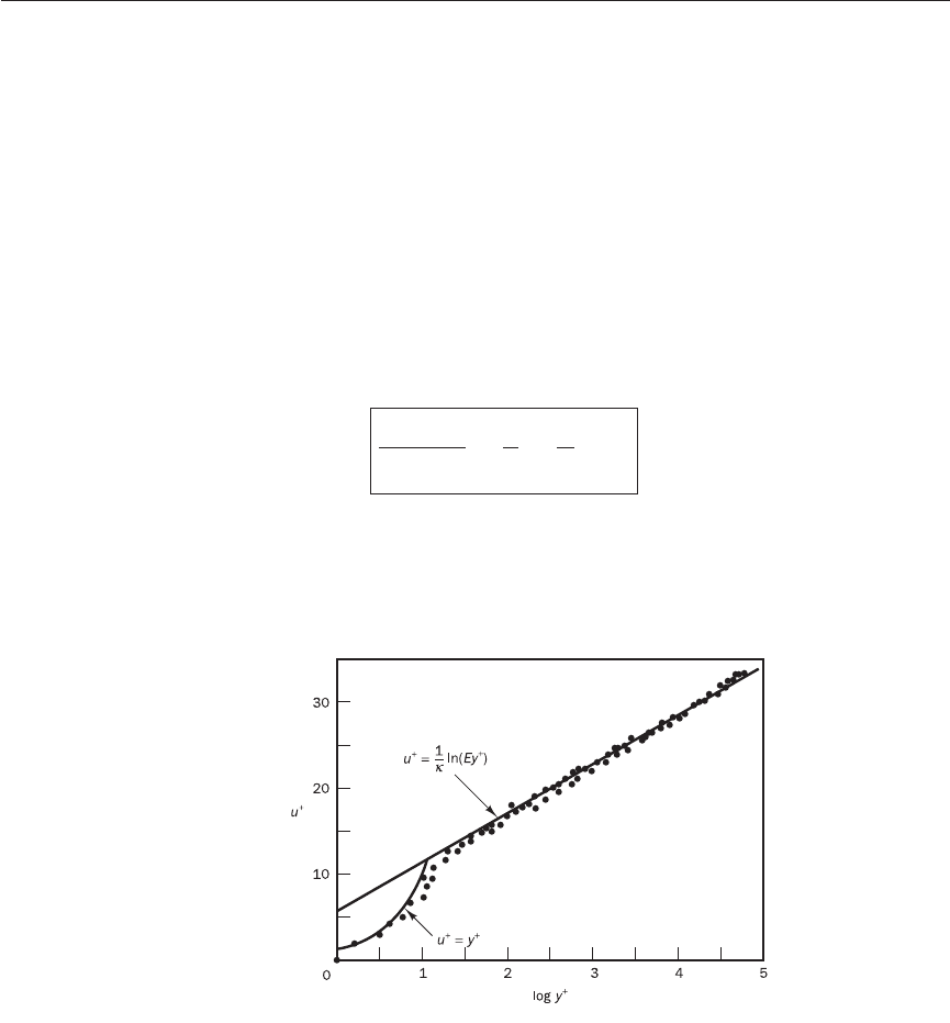
3.4 CHARACTERISTICS OF SIMPLE TURBULENT FLOWS 59

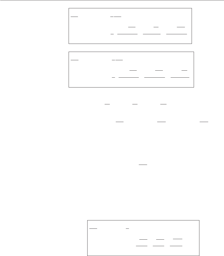
Figure 3.11 Velocity

distribution near a solid wall

Source: Schlichting, H. (1979)

Boundary Layer Theory, 7th edn,

reproduced with permission of

The McGraw-Hill Companies

Numerical values for the constants are found from measurements. We ﬁnd

von Karman’s constant

≈ 0.4 and the additive constant B ≈ 5.5 (or E ≈ 9.8)

for smooth walls; wall roughness causes a decrease in the value of B. The

values of

and B are universal constants valid for all turbulent ﬂows past

smooth walls at high Reynolds number. Because of the logarithmic relation-

ship between u

and y

, formula (3.18) is often called the log-law, and the

layer where y

takes values between 30 and 500 the log-law layer.

Outer layer --- the inertia-dominated region far from the wall

Experimental measurements show that the log-law is valid in the region

0.02 < y/

< 0.2. For larger values of y the velocity-defect law (3.17)

provides the correct form. In the overlap region the log-law and velocity-

defect law have to be equal. Tennekes and Lumley (1972) show that a

matched overlap is obtained by assuming the following logarithmic form:

=− ln + A (3.20)

where A is a constant. This velocity-defect law is often called the law of the

wake.

Figure 3.11 from Schlichting (1979) shows the close agreement between

theoretical equations (3.18) and (3.19) in their respective areas of validity and

experimental data.

max

− U

The turbulent boundary layer adjacent to a solid surface is composed of

two regions:

• The inner region: 10–20% of the total thickness of the wall layer;

the shear stress is (almost) constant and equal to the wall shear stress

Within this region there are three zones. In order of increasing distance

from the wall we have:

– the linear sub-layer: viscous stresses dominate the ﬂow adjacent to

surface

– the buffer layer: viscous and turbulent stresses are of similar magnitude

– the log-law layer: turbulent (Reynolds) stresses dominate.

ANIN_C03.qxd 29/12/2006 04:34PM Page 59

• The outer region or law-of-the-wake layer: inertia-dominated core ﬂow

far from wall; free from direct viscous effects.

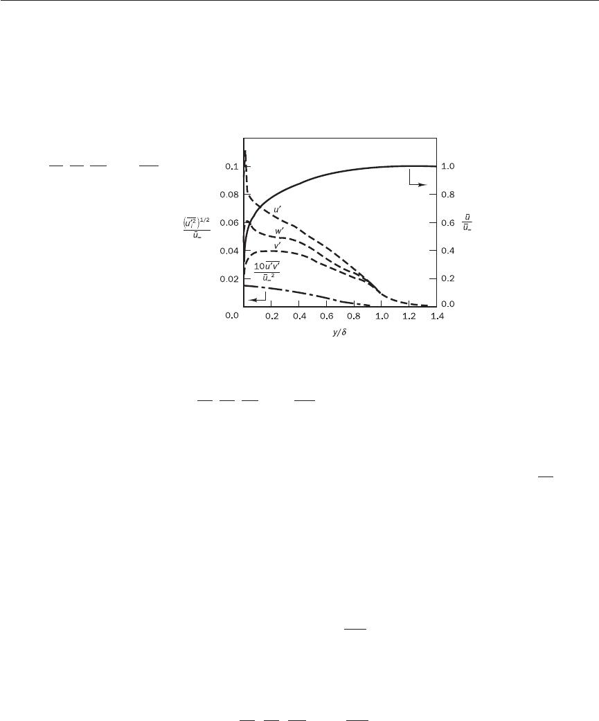
Figure 3.12 shows the mean velocity and turbulence property distribution

data for a ﬂat plate boundary layer with a constant imposed pressure

(Klebanoff, 1955).

60 CHAPTER 3 TURBULENCE AND ITS MODELLING

Figure 3.12 Distribution of

mean velocity and second

moments , , and −

for ﬂat plate boundary layer

u′v′w′

v′

u′

The mean velocity is at a maximum far away from the wall and sharply

decreases in the region y/

≤ 0.2 due to the no-slip condition. High values

of , , and − are found adjacent to the wall where the large mean

velocity gradients ensure that turbulence production is high. The eddying

motions and associated velocity ﬂuctuations are, however, also subject to

the no-slip condition at the wall. Therefore all turbulent stresses decrease

sharply to zero in this region. The turbulence is strongly anisotropic near

the wall since the production process mainly creates component . This is

borne out by the fact that this is the largest of the mean-squared ﬂuctuations

in Figure 3.12.

In the case of the ﬂat plate boundary layer the turbulence properties

asymptotically tend towards zero as y/

increases above a value of 0.8.

The r.m.s. values of all ﬂuctuating velocities become almost equal here, indi-

cating that the turbulence structure becomes more isotropic far away from

the wall. In pipe ﬂows, on the other hand, the eddying motions transport

turbulence across the centreline from areas of high production. Therefore,

the r.m.s. ﬂuctuations remain comparatively large in the centre of a pipe.

By symmetry the value of − has to go to zero and change sign at the

centreline.

This multi-layer structure is a universal feature of turbulent boundary

layers near solid surfaces. Monin and Yaglom (1971) plotted data from

Klebanoff (1955) and Laufer (1952) in the near-wall region and found not

only the universal mean velocity distribution but also that data for second

moments , , and − for ﬂat plates and pipes collapse onto a

single curve if they are non-dimensionalised with the correct velocity scale

. Between these distinct layers there are intermediate zones which ensure

that the various distributions merge smoothly. Interested readers may ﬁnd

further details including formulae which cover the whole inner region and

the log-law/law-of-the-wake layer in Schlichting (1979) and White (1991).

u′v′w

′

u′v′

′

u′v′w

′

ANIN_C03.qxd 29/12/2006 04:34PM Page 60

3.5 EFFECT OF FLUCTUATIONS ON THE MEAN FLOW 61

3.4.3 Summary

Our review of the characteristics of a number of two-dimensional turbulent

ﬂows revealed many common features. Turbulence is generated and main-

tained by shear in the mean ﬂow. Where shear is large the magnitudes of tur-

bulence quantities such as the r.m.s. velocity ﬂuctuations are high and their

distribution is anisotropic with higher levels of ﬂuctuations in the mean ﬂow

direction. Without shear, or an alternative agency to maintain it, turbulence

decays and becomes more isotropic in the process. In spite of these common

features, it was clear that, even in these relatively simple thin shear layers,

the details of the turbulence structure are very much dependent on the ﬂow

itself. In regions close to solid walls the structure is dominated by shear due

to wall friction and damping of turbulent velocity ﬂuctuations perpendicular

to the boundary. This results in a complex ﬂow structure characterised by

rapid changes in the mean and ﬂuctuating velocity components concentrated

within a very narrow region in the immediately vicinity of the wall. Since

most engineering ﬂows contain solid boundaries, the turbulence structure

generated by them will be very geometry dependent. Engineering ﬂow cal-

culations must include sufﬁciently accurate and general descriptions of the

turbulence that capture all the above effects and further interactions of

turbulence and body forces.

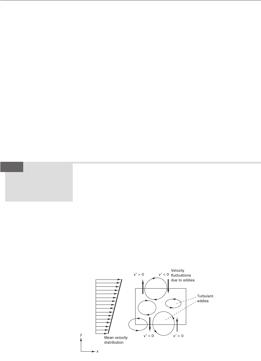
In this section we derive the ﬂow equations governing the time-averaged

properties of a turbulent ﬂow, but before we do this we brieﬂy examine the

physical basis of the effects resulting from the appearance of turbulent

ﬂuctuations.

In Figure 3.13 we consider a control volume in a two-dimensional turbu-

lent shear ﬂow parallel to the x-axis with a mean velocity gradient in the

y-direction. The presence of vortical eddy motions creates strong mixing.

Random currents that are associated with the passage of eddies near the

boundaries of the control volume transport ﬂuid across its boundaries. These

recirculating ﬂuid motions cannot create or destroy mass, but ﬂuid parcels

transported by the eddies will carry momentum and energy into and out of

the control volume. Figure 3.13 shows that, because of the existence of the

velocity gradient, ﬂuctuations with a negative y-velocity will generally bring

Figure 3.13 Control volume

within a two-dimensional

turbulent shear ﬂow

The effect of

turbulent

fluctuations

on properties of

the mean flow

3.5

ANIN_C03.qxd 29/12/2006 04:34PM Page 61

ﬂuid parcels with a higher x-momentum into the control volume across

its top boundary and will also transport control volume ﬂuid to a region

of slower moving ﬂuid across the bottom boundary. Similarly, positive y-

velocity ﬂuctuations will – on average – transport slower moving ﬂuid into

regions of higher velocity. The net result is momentum exchange due to

convective transport by the eddies, which causes the faster moving ﬂuid

layers to be decelerated and the slower moving layers to be accelerated.

Consequently, the ﬂuid layers experience additional turbulent shear stresses,

which are known as the Reynolds stresses. In the presence of temperature

or concentration gradients the eddy motions will also generate turbulent

heat or species concentration ﬂuxes across the control volume bound-

aries. This discussion suggests that the equations for momentum and energy

should be affected by the appearance of ﬂuctuations.

Reynolds-averaged Navier---Stokes equations for

incompressible flow

Next we examine the consequences of turbulent ﬂuctuations for the mean

ﬂow equations for an incompressible ﬂow with constant viscosity. These

assumptions considerably simplify the algebra involved without detracting

from the main messages. We begin by summarising the rules which govern

time averages of ﬂuctuating properties

=Φ+

′ and

=Ψ+

′ and their

summation, derivatives and integrals:

==0 =Φ = = Φds (3.21)

=Φ+Ψ =ΦΨ+ =ΦΨ =0

These relationships can be easily veriﬁed by application of (3.2) and (3.3),

noting that the time-averaging operation is itself an integration. Thus, the

order of time averaging and summation, further integration and/or differen-

tiation can be swapped or commuted, so this is called the commutative

property.

Since div and grad are both differentiations, the above rules can be

extended to a ﬂuctuating vector quantity a = A + a′ and its combinations

with a ﬂuctuating scalar

=Φ+

′:

= div A; = div( ) = div(ΦA) + div( );

= div grad Φ (3.22)

To start with we consider the instantaneous continuity and Navier–Stokes

equations in a Cartesian co-ordinate system so that the velocity vector u has

x-component u, y-component v and z-component w:

div u = 0 (3.23)

+ div(uu) =− +

div(grad(u)) (3.24a)

+ div(vu) =− +

div(grad(v)) (3.24b)

+ div(wu) =− +

div(grad(w)) (3.24c)

∂

div grad

′a′

adiv(

a)div a

′Ψ

′

ϕψϕ



∂

∂ϕ

∂

′

62 CHAPTER 3 TURBULENCE AND ITS MODELLING

ANIN_C03.qxd 29/12/2006 04:34PM Page 62

3.5 EFFECT OF FLUCTUATIONS ON THE MEAN FLOW 63

This system of equations governs every turbulent ﬂow, but we investigate

the effects of ﬂuctuations on the mean ﬂow using the Reynolds decomposi-

tion in equations (3.23) and (3.24a–c) and replace the ﬂow variables u (hence

also u, v and w) and p by the sum of a mean and ﬂuctuating component. Thus

u = U + u′ u = U + u′ v = V + v′ w = W + w′ p = P + p′

Then the time average is taken, applying the rules stated in (3.21)–(3.22).

Considering the continuity equation (3.23), ﬁrst we note that = div U.

This yields the continuity equation for the mean ﬂow:

div U = 0 (3.25)

A similar process is now carried out on the x-momentum equation (3.24a). The

time averages of the individual terms in this equation can be written as follows:

==div(UU) + div( )

−=− =

div(grad(U))

Substitution of these results gives the time-average x-momentum equation

+ div(UU) + div( ) =− +

div(grad(U)) (3.26a)

(I) (II) (III) (IV) (V)

Repetition of this process on equations (3.24b) and (3.24c) yields the time-

average y- and z-momentum equations:

+ div(V U) + div( ) =− +

div(grad(V)) (3.26b)

(I) (II) (III) (IV) (V)

+ div(W U) + div( ) =− +

div(grad(W)) (3.26c)

(I) (II) (III) (IV) (V)

It is important to note that the terms (I), (II), (IV) and (V) in (3.26a–c) also

appear in the instantaneous equations (3.24a–c), but the process of time

averaging has introduced new terms (III) in the resulting time-average

momentum equations. The terms involve products of ﬂuctuating velocities

and are associated with convective momentum transfer due to turbulent

eddies. It is customary to place these terms on the right hand side of equa-

tions (3.26a–c) to reﬂect their role as additional turbulent stresses on the

mean velocity components U, V and W:

+ div(UU) =− +

div(grad(U))

+++ (3.27a)

∂

(−

u′w′)

∂

(−

u′v′)

∂

(−

u′

)

∂

w′u′

∂

v′u′

∂

u′u′

∂

div(grad(u))

∂

u′u′div(uu)

∂

div u

ANIN_C03.qxd 29/12/2006 04:34PM Page 63

64 CHAPTER 3 TURBULENCE AND ITS MODELLING

+ div(V U) =− +

div(grad(V))

+++ (3.27b)

+ div(W U) =− +

div(grad(W))

+++ (3.27c)

The extra stress terms have been written out in longhand to clarify their

structure. They result from six additional stresses: three normal stresses

=−

=− (3.28a)

and three shear stresses

=−

=− (3.28b)

These extra turbulent stresses are called the Reynolds stresses. The

normal stresses involve the respective variances of the x-, y- and z-velocity

ﬂuctuations. They are always non-zero because they contain squared velo-

city ﬂuctuations. The shear stresses contain second moments associated with

correlations between different velocity components. As was stated earlier,

if two ﬂuctuating velocity components, e.g. u′ and v′, were independent ran-

dom ﬂuctuations the time average would be zero. However, the correla-

tion between pairs of different velocity components due to the structure of

the vortical eddies ensures that the turbulent shear stresses are also non-zero

and usually very large compared with the viscous stresses in a turbulent ﬂow.

The equation set (3.25) and (3.27a–c) is called the Reynolds-averaged

Navier–Stokes equations.

Similar extra turbulent transport terms arise when we derive a transport

equation for an arbitrary scalar quantity, e.g. temperature. The time-average

transport equation for scalar

ϕϕ

+ div(ΦU) = div(Γ

grad Φ)

+− − − +S

(3.29)

So far we have assumed that the ﬂuid density is constant, but in practical

ﬂows the mean density may vary and the instantaneous density always

exhibits turbulent ﬂuctuations. Bradshaw et al. (1981) stated that small

density ﬂuctuations do not appear to affect the ﬂow signiﬁcantly. If r.m.s.

velocity ﬂuctuations are of the order of 5% of the mean speed they show that

density ﬂuctuations are unimportant up to Mach numbers around 3 to 5. In

free turbulent ﬂows we have seen in section 3.4 that velocity ﬂuctuations can

easily reach values around 20% of the mean velocity. In such circumstances

∂

w′

′

∂

v′

′

∂

u′

′

∂

u′v′

v′w′

u′w′

u′v′

w′

v′

u′

∂

(−

w′

)

∂

(−

v′w′)

∂

(−

u′w′)

∂

(−

v′w′)

∂

(−

v′

)

∂

(−

u′v′)

∂

ANIN_C03.qxd 29/12/2006 04:34PM Page 64

3.6 TURBULENT FLOW CALCULATIONS 65

density ﬂuctuations start to affect the turbulence around Mach numbers

of 1. To summarise the results of the current section we quote, without

proof, in Table 3.1, the density-weighted averaged (or Favre-averaged;

see Anderson et al., 1984) form of the mean ﬂow equations for compressible

turbulent ﬂows where effects of density ﬂuctuations are negligible, but mean

density variations are not. This form is widely used in commercial CFD

packages. The symbol } stands for the Favre-averaged velocity.

Table 3.1 Turbulent ﬂow equations for compressible ﬂows

Continuity + div(4-) = 0 (3.30)

Reynolds equations

+ div(4}-) =− +div(

grad }) + − − − + S

(3.31a)

+ div(4I -) =− +div(

grad I ) + − − − + S

(3.31b)

+ div(4| -) =− +div(

grad | ) +− − − +S

(3.31c)

Scalar transport equation

+ div(45-) = div(Γ

grad 5) +− − − +S

(3.32)

where the overbar indicates a time-averaged variable and the tilde indicates a density-weighted or Favre-averaged

variable

∂

(4w′

′)

∂

(4v′

′)

∂

(4u′

′)

∂

(45)

∂

(4w′

)

∂

(4v′w′)

∂

(4u′w′)

∂

(4|)

∂

(4v′w′)

∂

(4v′

)

∂

(4u′v′)

∂

(4I)

∂

(4u′w′)

∂

(4u′v′)

∂

(4u′

)

∂

(4})

∂

Turbulent flow

calculations

Turbulence causes the appearance in the ﬂow of eddies with a wide range of

length and time scales that interact in a dynamically complex way. Given the

importance of the avoidance or promotion of turbulence in engineering

applications, it is no surprise that a substantial amount of research effort is

dedicated to the development of numerical methods to capture the important

effects due to turbulence. The methods can be grouped into the following

three categories:

• Turbulence models for Reynolds-averaged Navier–Stokes

(RANS) equations: attention is focused on the mean ﬂow and the

effects of turbulence on mean ﬂow properties. Prior to the application

of numerical methods the Navier–Stokes equations are time averaged

(or ensemble averaged in ﬂows with time-dependent boundary

conditions). Extra terms appear in the time-averaged (or Reynolds-

averaged) ﬂow equations due to the interactions between various

turbulent ﬂuctuations. These extra terms are modelled with classical

turbulence models: among the best known ones are the k–

model and

3.6

ANIN_C03.qxd 29/12/2006 04:34PM Page 65

the Reynolds stress model. The computing resources required for

reasonably accurate ﬂow computations are modest, so this approach

has been the mainstay of engineering ﬂow calculations over the last

three decades.

• Large eddy simulation: this is an intermediate form of turbulence

calculations which tracks the behaviour of the larger eddies. The

method involves space ﬁltering of the unsteady Navier–Stokes

equations prior to the computations, which passes the larger eddies

and rejects the smaller eddies. The effects on the resolved ﬂow (mean

ﬂow plus large eddies) due to the smallest, unresolved eddies are

included by means of a so-called sub-grid scale model. Unsteady

ﬂow equations must be solved, so the demands on computing resources

in terms of storage and volume of calculations are large, but (at the time

of writing) this technique is starting to address CFD problems with

complex geometry.

• Direct numerical simulation (DNS): these simulations compute

the mean ﬂow and all turbulent velocity ﬂuctuations. The unsteady

Navier–Stokes equations are solved on spatial grids that are sufﬁciently

ﬁne that they can resolve the Kolmogorov length scales at which energy

dissipation takes place and with time steps sufﬁciently small to resolve

the period of the fastest ﬂuctuations. These calculations are highly

costly in terms of computing resources, so the method is not used for

industrial ﬂow computations.

In the next section we discuss the main features and achievements of each of

these methods.

For most engineering purposes it is unnecessary to resolve the details of

the turbulent ﬂuctuations. CFD users are almost always satisﬁed with infor-

mation about the time-averaged properties of the ﬂow (e.g. mean velocities,

mean pressures, mean stresses etc.). Therefore, the vast majority of turbu-

lent ﬂow computations has been and for the foreseeable future will continue

to be carried out with procedures based on the Reynolds-averaged

Navier–Stokes (RANS) equations (3.30), (3.31a–c) and (3.32). A descrip-

tion of the effects of turbulence on the mean ﬂow is nevertheless needed

because the time-averaging operation on the momentum equations discards

all details concerning the state of the ﬂow contained in the instantaneous

ﬂuctuations. We have already seen in section 3.5 that this yields six addi-

tional unknowns in the time-averaged momentum equations (3.31a–c): the

Reynolds stresses −

, −

. Similarly,

time-average scalar transport equations show extra terms containing ,

and .

In order to be able to compute turbulent ﬂows with the RANS equations

it is necessary to develop turbulence models to predict the Reynolds

stresses and the scalar transport terms and close the system of mean ﬂow

equations (3.30), (3.31a–c) and (3.32). For a turbulence model to be useful in

a general-purpose CFD code it must have wide applicability, be accurate,

simple and economical to run. The most common RANS turbulence models

are classiﬁed on the basis of the number of additional transport equations

that need to be solved along with the RANS ﬂow equations:

w′

′v′

′

u′

′

v′w′u′w′u′v′w′

v′

u′

66 CHAPTER 3 TURBULENCE AND ITS MODELLING

Reynolds-

averaged Navier---

Stokes equations

and classical

turbulence models

3.7

ANIN_C03.qxd 29/12/2006 04:34PM Page 66