Alligood K., Sauer T., Yorke J.A. Chaos: An Introduction to Dynamical Systems
Подождите немного. Документ загружается.


C HAOTIC ATTRACTORS
✎ E XERCISE T6.10
Let f be a map of the interval I for which almost every orbit is attracted by
aperiod-k sink. Find the natural measure of f and justify your answer.
6.6 INVARIANT MEASURE FOR
ONE-DIMENSIONAL MAPS
In this section we show how to find invariant measures, and in some cases natural
measures, for a class of one-dimensional maps. We will call a map f on [0, 1]
piecewise smooth if f(x),f
(x), and f
(x) are continuous and bounded except
possibly at a finite number of points. Recall that a map is piecewise expanding if
furthermore there is some constant
␣
⬎ 1suchthat|f
(x)| ⱖ
␣
except at a finite
number of points in [0, 1]. Example 6.12 and the W-map of Example 6.10 satisfy
these conditions.
✎ E XERCISE T6.11
Verify that the following maps on [0, 1] are piecewise expanding. (a)The
piecewise linear map f (x) ⫽ a ⫹ bx mod 1, where a ⱖ 0andb ⬎ 1. (b) The
tent map T
b
(x) with slopes ⫾b,where1⬍ b ⱕ 2.
Theorem 6.15 Assume that the map f on [0, 1] is piecewise smooth and
piecewise expanding. Then f has an invariant measure
. Furthermore the density is
bounded, meaning that there is a constant c such that
([a, b]) ⱕ c|b ⫺ a| for every
0 ⱕ a ⬍ b ⱕ 1.
The proof of this theorem is beyond the scope of this book (see (Lasota
and Yorke, 1973) and (Li and Yorke, 1978)). Next we give some particularly
nice examples for which
can be exactly determined. It is possible for piecewise
expanding maps to have more than one attractor, in which case each attractor will
have a natural measure. We will see that for some choices of [a, b], it is possible
that
([a, b]) ⫽ 0.
In the examples we discuss, invariant measures have a simple description as
the integral of a piecewise constant nonnegative function. That means that the
measure of a subset S of I will be given by
(S) ⫽
S
p(x) dx
256
6.6 INVARIANT M EASURE FOR O NE-DIMENSIONAL M APS
for some
p(x) ⫽
p
1
if x 僆 A
1
.
.
.
p
n
if x 僆 A
n
,
where the p
i
ⱖ 0and
n
i⫽1
p
i
length(A
i
) ⫽ 1. When the measure of a set is given
by the integral of a function over the set, such as the relationship between the
measure
and the function p in this case, then the function p is called the density
of the measure.
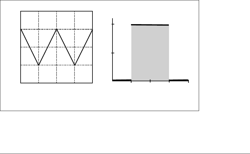
For example, consider the W-map, shown in Figure 6.12 along with the
density that defines its invariant measure:
p(x) ⫽
p
1
⫽ 0if0ⱕ x ⬍ 1 4
p
2
⫽ 2if1 4 ⱕ x ⬍ 1 2
p
3
⫽ 2if1 2 ⱕ x ⬍ 3 4
p
4
⫽ 0if3 4 ⱕ x ⱕ 1
. (6.8)
Notice that the function p(x) is the density of a probability measure, since
1
0
p(x) dx ⫽ 1. This measure is invariant under the W-map f because
(S) ⫽
S
p(x) dx ⫽
f
⫺1
(S)
p(x) dx ⫽
(f
⫺1
(S))
0 1/2
1
1/2
1
A
1
A
2
A
3
A
4
1
2
0 1/2
1
(a) (b)
Figure 6.12 The W-map.
(a) The map is linear on each of four subintervals. (b) The density p(x) that defines
the invariant measure of (a). According to this graph, the measure of an interval
inside [1 4, 3 4] is twice its length.
257

C HAOTIC ATTRACTORS
for each set S.LetS ⫽ [1 4, 3 8] for purposes of illustration. Then f
⫺1
(S) ⫽
[3 16, 5 16] 傼 [11 16, 13 16], as can be checked using Figure 6.12. The
-
measure of S is
(S) ⫽
S
p(x) dx ⫽
3 8
1 4
2 dx ⫽ 2(3 8 ⫺ 1 4) ⫽ 1 4,
which is the same as
(f
⫺1
(S)) ⫽
f
⫺1
(S)
p(x) dx
⫽
4 16
3 16
0 dx ⫹
5 16
4 16
2 dx ⫹
12 16
11 16
2 dx ⫹
13 16
12 16
0 dx
⫽ 0 ⫹ 1 8 ⫹ 1 8 ⫹ 0. (6.9)
As another example, assume instead that S is completely contained in [0, 1 4].
No points map to it, so f
⫺1
(S) is the empty set, which must have measure zero as
required by the definition of measure. We can state this as a general fact.
✎ E XERCISE T6.12
Let f be a map on the interval I and let
be an invariant measure for f .
Show that if S is a subset of I that is outside the range of f ,then
(S) ⫽ 0.
✎ E XERCISE T6.13
Prove that
(S) ⫽
(f
⫺1
(S)) for the invariant measure
of the W-map,
for any subset S of the unit interval.
Next we show how to calculate the invariant measures for expanding
piecewise-linear maps of the interval. In general we assume that the interval
is the union of subintervals A
1
,...,A
k
, and that the map f has constant slope s
i
on subinterval A
i
. We also assume that the image of each A
i
under f is exactly a
union of some of the subintervals. Define the Z-matrix of f to be a k ⫻ k matrix
whose (i, j) entry is the reciprocal of the absolute value of the slope of the map
from A
j
to A
i
,orzeroifA
j
does not map across A
i
. For the W-map, defined in four
subintervals A
1
,A
2
,A
3
,A
4
, the Z-matrix is
Z ⫽
0000
1 21 21 21 2
1 21 21 21 2
0000
. (6.10)
258
6.6 INVARIANT M EASURE FOR O NE-DIMENSIONAL M APS
As we explain below, a Z-matrix has no eigenvalues greater than 1 in
magnitude, and 1 is always an eigenvalue. Any eigenvector x ⫽ (x
1
,...,x
k
)
associated to the eigenvalue 1 corresponds to an invariant measure of f,when
properly normalized so that the total measure is 1. The normalization is done by
dividing x by x
1
L
1
⫹⭈⭈⭈⫹x
k
L
k
,whereL
i
is the length of A
i
.Theith component
of the resulting eigenvector gives the height of the density p
i
on A
i
.
For example, the Z-matrix (6.10) for the W-map has characteristic polyno-
mial P(
) ⫽
3
(
⫺ 1) and eigenvalues 1,0,0,0. All eigenvectors associated with
the eigenvalue 1 are scalar multiples of x ⫽ (0, 1, 1, 0). Normalization entails
dividing x by 0 ⭈ 1 4 ⫹ 1 ⭈ 1 4 ⫹ 1 ⭈ 1 4 ⫹ 0 ⭈ 1 4 ⫽ 1 2, yielding the den-
sity p ⫽ (0, 2, 2, 0) of Equation (6.8). Because the other eigenvalues are 0, the
measure defined by this density is a natural measure for the W-map.
There may be several different invariant measures for f if the space of
eigenvectors associated to the eigenvalue 1 has dimension greater than one. An
eigenvalue is called simple if this is not the case, if there is only a one-dimensional
space of eigenvectors. If 1 is a simple eigenvalue and if all other eigenvalues of
the Z-matrix are strictly smaller than 1 in magnitude, then the resulting measure
is a natural measure for f, meaning that almost every point in the interval will
generate this measure.
Next we explain why the Z-matrix procedure works. Let p
i
be the total den-
sity of the invariant measure on A
i
, assumed to be constant on the subinterval.
The amount of measure contained in A
i
is L
i
p
i
. Since the slope of f is constant
on A
i
, one iteration of the map distributes this measure evenly over other subin-
tervals. The image of A
i
has length s
i
L
i
,wheres
i
is the absolute value of the slope
of the map on A
i
. Therefore the proportion of A
i
’s measure deposited into A
j
is
L
j
(L
i
s
i
). (For the W-map, the s
i
are all 2.) Since the p
i
represent the density of
an invariant measure by assumption, the total measure mapped into A
j
from all
A
i
’s must total up to L
j
p
j
. For the W-map this can be summarized in the matrix
equation
0000
L
2
L
1
s
1
L
2
L
2
s
2
L
2
L
3
s
3
L
2
L
4
s
4
L
3
L
1
s
1
L
3
L
2
s
2
L
3
L
3
s
3
L
3
L
4
s
4
0000
L
1
p
1
L
2
p
2
L
3
p
3
L
4
p
4
⫽
L
1
p
1
L
2
p
2
L
3
p
3
L
4
p
4
. (6.11)
Since the L
i
are known, finding the invariant measure 兵p
i
其 is equivalent to finding
an eigenvector of the matrix in (6.11) with eigenvalue 1. This matrix turns out
to have some interesting properties. For example, notice that each column adds
up to exactly 1. That is because the length of the image f(A
i
)iss
i
L
i
,sothe
numerators in each column must add up to s
i
L
i
.
259
C HAOTIC ATTRACTORS
Definition 6.16 A square matrix with nonnegative entries, whose
columns each add up to 1, is called a Markov matrix.
A Markov matrix always has the eigenvalue
⫽ 1, and its corresponding
eigenvector has nonnegative entries. If the remaining eigenvalues are smaller than
1 in magnitude, then all vectors except linear combinations of eigenvectors of the
other eigenvalues tend to the dominant eigenvector upon repeated multiplication
by the matrix. See, for example, (Strang, 1988). In our application, when this
eigenvector is normalized so that the sum of its entries is 1, its ith entry is the
amount of measure L
i
p
i
in A
i
.
We can simplify (6.11) quite a bit by defining
D ⫽
L
1
.
.
.
L
k
,p⫽
p
1
.
.
.
p
k
.
It is a fact that multiplying a matrix by a diagonal matrix diag(L
1
,...,L
k
)on
the left results in multiplying the ith row by L
i
, while multiplying by a diagonal
matrix on the right multiplies the ith column by L
i
. Then (6.11) can be written
DZD
⫺1
Dp ⫽ Dp, which simplifies to Zp ⫽ p by multiplying both sides by D
⫺1
on the left. This concludes our explanation since it shows that solving for an
eigenvector of Z with eigenvalue 1 will give an invariant measure.
✎ E XERCISE T6.14
Show that the Z-matrix for the tent map is
1
2
1
2
1
2
1
2
, and that the density
which defines the natural measure is the constant p(x) ⫽ 1on[0, 1]. Thus
the natural measure for this map is ordinary Lebesgue (length) measure.
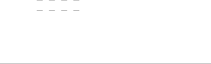
E XAMPLE 6.17
(Critical point is period-three.) Recall the map from Example 6.12, shown
in Figure 6.10(a). The Z-matrix is
0
1
a
1
a
1
a
, (6.12)
where a ⫽ (
5 ⫹ 1) 2 satisfies a
2
⫽ a ⫹ 1. The characteristic equation is
2
⫺ (1 a)
⫺ 1 a
2
⫽ 0. We know (
⫺ 1) is a factor, and so the factoriza-
260
6.6 INVARIANT M EASURE FOR O NE-DIMENSIONAL M APS
tion (
⫺ 1)(
⫹ c) ⫽ 0 follows, where c ⫽ 1 a
2
⬇ 0.382. The eigenvalues are
1and⫺c. Since the latter is smaller than 1 in absolute value, there is a natural
measure. An eigenvector associated to 1 is (x
1
,x
2
) ⫽ (1,a). The normalization
involves dividing this eigenvector by x
1
L
1
⫹ x
2
L
2
⫽ 1 ⭈ c ⫹ a ⭈ (1 ⫺ c). The result
is that the natural measure for f is
(S) ⫽
S
p(x) dx,where
p(x) ⫽
1 ⫺ 1 (1 ⫹ a
2
)if0ⱕ x ⱕ c
a ⫺ a (1 ⫹ a
2
)ifc ⱕ x ⱕ 1
.
The measure is illustrated in Figure 6.10(c).
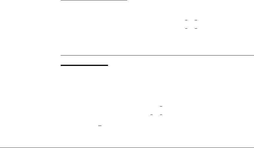
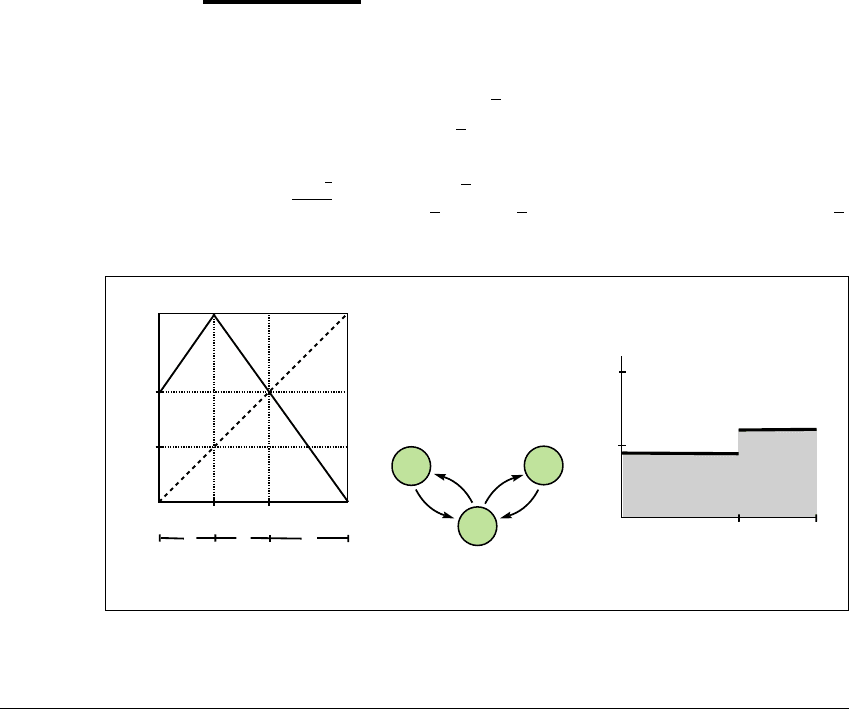
E XAMPLE 6.18
Let
f(x) ⫽
1
2
⫺ 2x if 0 ⱕ x ⱕ
1
4
⫺
1
2
⫹ 2x if
1
4
ⱕ x ⱕ
3
4
5
2
⫺ 2x if
3
4
ⱕ x ⱕ 1
,
as shown in Figure 6.13. The transition graph is shown in Figure 6.13(b).
There is a stretching partition 0 ⬍ 1 4 ⬍ 1 2 ⬍ 3 4 ⬍ 1, but no dense
orbit, because A
1
and A
4
cannot be connected by an itinerary. There are, however,
0 1/2
1
1/2
1
A
1
A
2
A
3
A
4
A
1
A
2
A
3
A
4
0
1
1
2
1/2
q
2-q
(a) (b) (c)
Figure 6.13 A piecewise linear map with no dense orbit.
(a) Sketch of map. (b) Transition graph. (c) One invariant measure for (a). In this
case, there is no unique invariant measure—there are infinitely many.
261
C HAOTIC ATTRACTORS
dense orbits for the map restricted to [0, 1 2] and to [1 2, 1]. The Z-matrix is
Z ⫽
1 21 20 0
1 21 20 0
001 21 2
001 21 2
.
The eigenvalues of Z are 1, 1, 0, 0. Both (2, 2, 0, 0) and (0, 0, 2, 2), as well as
linear combinations of them, are eigenvectors associated to 1. As a result, there
are many invariant measures for f: for any 0 ⬍ q ⬍ 1, the measure defined by
p(x) ⫽
q if 0 ⱕ x ⱕ 1 2
2 ⫺ q if 1 2 ⱕ x ⱕ 1
.
is invariant. The map has no natural measure.
E XAMPLE 6.19
(Critical point eventually maps onto fixed point.) Let
f(x) ⫽
2 ⫹
2(x ⫺ 1) if 0 ⱕ x ⱕ c
2(1 ⫺ x)ifc ⱕ x ⱕ 1
,
where c ⫽
2⫺
2
2
and d ⫽ 2 ⫺
2 is a fixed point of f. See Figure 6.14. Check that
the slopes of the map are
2and⫺
2. The stretching factor for f is
␣
⫽
2,
0
1
1
c
c
A B
d
d
C
A
B
C
0
1
1
2
d
(a) (b) (c)
Figure 6.14 Map in which the critical point is eventually periodic.
(a) Sketch of map. (b) Transition graph. (c) Invariant measure for (a).
262

6.6 INVARIANT M EASURE FOR O NE-DIMENSIONAL M APS
and the Lyapunov exponent is ln
2 for each orbit for which it is defined. The
transition graph is shown in Figure 6.14(b).
Notice that f
3
(c) ⫽ d, so that the critical point is an eventually fixed
point. The partition 0 ⬍ c ⬍ d ⬍ 1 is a stretching partition for f. Define the
subintervals A ⫽ (0,c),B ⫽ (c, d), and C ⫽ (d, 1). Then f(A) ⫽ C, f(B) ⫽ C,
and f(C) ⫽ A 傼 B. Check that all pairs of symbols can be connected. According
to Theorem 6.11, f has a dense chaotic orbit on I,andI is a chaotic attractor for f.
The Z-matrix is
Z ⫽
001
␣
001
␣
1
␣
1
␣
0
,
where the stretching factor for f is
␣
⫽
2. The eigenvectors of this matrix are
1, ⫺1, and 0. The invariant measure associated to the eigenvalue 1 turns out to
be a natural measure. Check that the measure is defined by
p(x) ⫽
1 (2d)if0ⱕ x ⱕ d
1 (
2d)ifd ⱕ x ⱕ 1
. (6.13)
➮ COMPUTER EXPERIMENT 6.3
Write a computer program to approximate the natural measure of an interval
map. Divide the interval into equally-spaced bins, and count the number of points
that fall into each bin from a given orbit. Calculate the natural measure for
Example 6.19 and compare with (6.13). Then calculate the natural measure for
the logistic map and compare to the answer in Challenge 6.
263
C HAOTIC ATTRACTORS
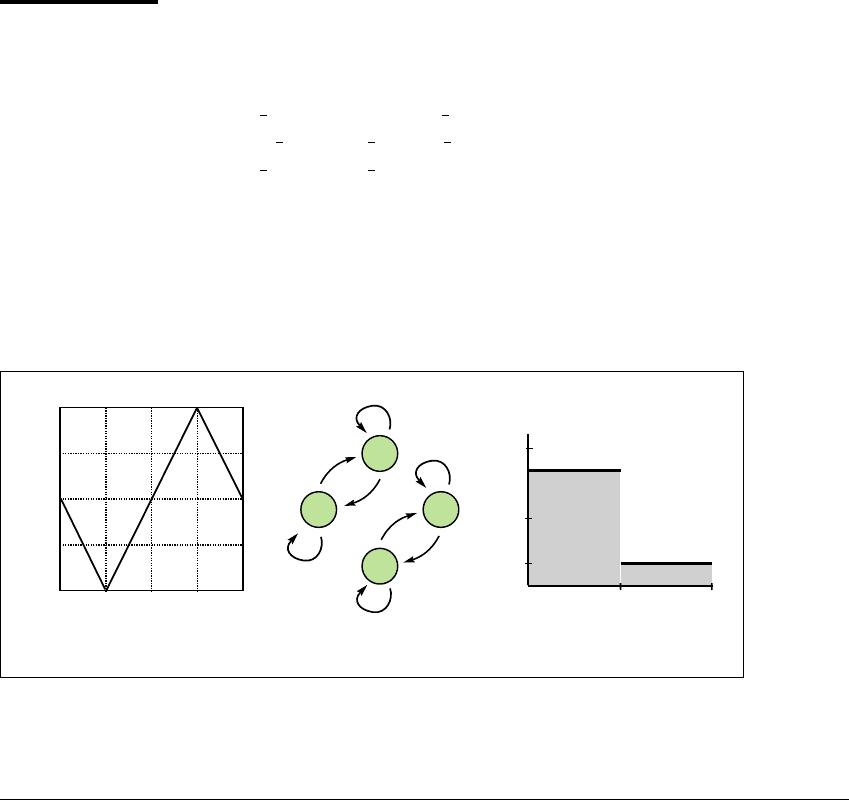
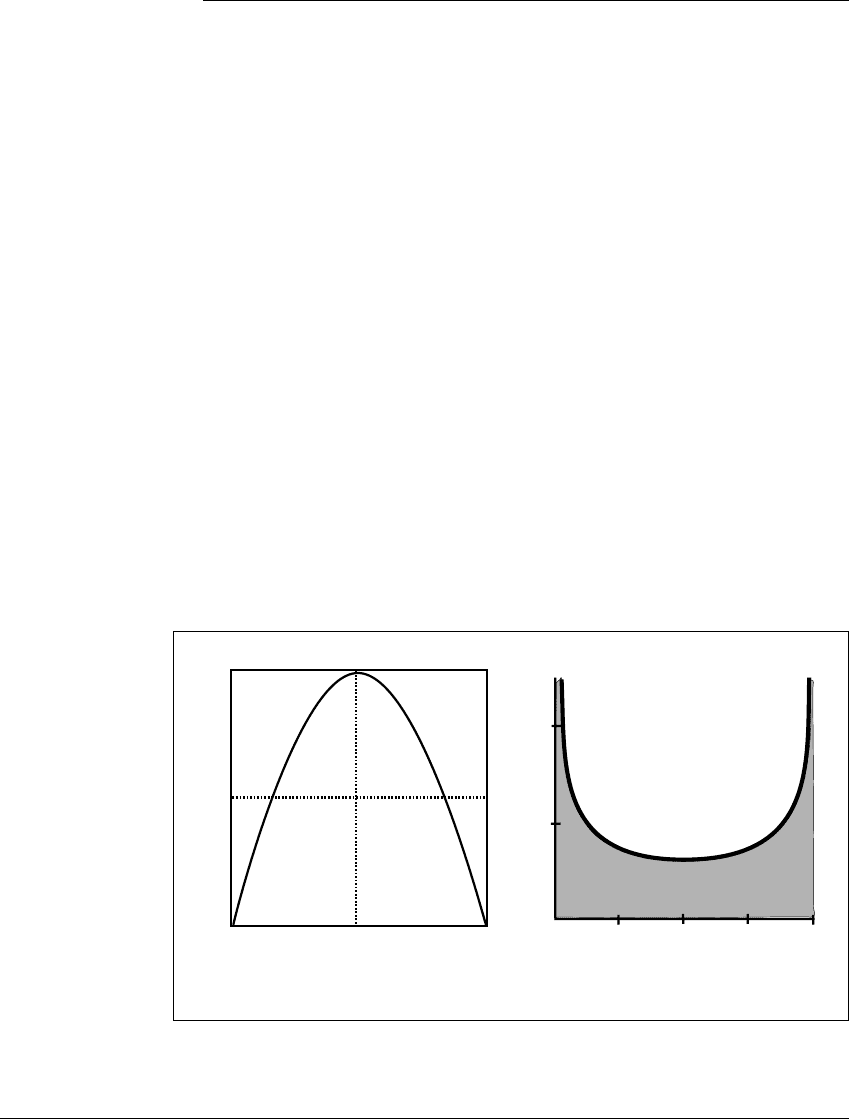
☞ C HALLENGE 6
Invariant Measure for the Logistic Map
W
E HAVE SEEN how to construct invariant measures for simple piecewise
linear maps of the interval. More complicated maps can be significantly more
difficult. In Challenge 6 you will work out the invariant measure of the logistic
map G(x) ⫽ 4x(1 ⫺ x).
In Chapter 3 we found a conjugacy C(x) ⫽ (1 ⫺ cos
x) 2 between the
tent map T ⫽ T
2
and the logistic map, satisfying CT ⫽ GC. Exercise T6.14 shows
the invariant measure of the tent map to be m
1
, ordinary length measure on the
unit interval. Some elementary calculus will allow the transfer of the invariant
measure of the tent map to one for the logistic map.
Step 1 If S is a subset of the unit interval, prove that the sets T
⫺1
(S)
and C
⫺1
G
⫺1
C(S) are identical. (Remember that T and G are not invertible; by
T
⫺1
(S) we mean the points x such that T(x) lies in S.)
Step 2 Use the fact that m
1
is invariant for the tent map to prove that
m
1
(S) ⫽ m
1
(C
⫺1
G
⫺1
C(S)) for any subset S.
0 1/2
1
1
1
2
0 1/2
1
(a) (b)
Figure 6.15 The logistic map
G
.
(a) Sketch of map. (b) The invariant measure for G.
264

C HALLENGE 6
Step 3 Prove that the the definition
(S) ⫽ m
1
(C
⫺1
(S)) results in a
probability measure
on the unit interval.
Step 4 Use Step 2 to show that
is an invariant measure for G.
Step 5 It remains to compute the density p(x). So far we know
(S) ⫽
C
⫺1
(S)
1 dx.
Using the change of variable y ⫽ (1 ⫺ cos
x) 2, rewrite
(S) as an integral
S
p(y) dy
in y over the set S, and find the density p(y). See Figure 6.15(b) for a graph of
p(x). (Answer: p(x) ⫽ 1
x ⫺ x
2
)
265