Alligood K., Sauer T., Yorke J.A. Chaos: An Introduction to Dynamical Systems
Подождите немного. Документ загружается.


C HAOTIC ATTRACTORS
E XERCISES
6.1. Show that a chaotic attractor cannot contain a sink.
6.2. For each of the piecewise linear maps shown in Figures 6.10(a), 6.13(a), and 6.14(a),
find all periods for which there are periodic points.
6.3. Let f(x, y) ⫽ (
4
arctan x, y 2). Find all forward limit sets, attractors, and basins for
each attractor. What is the basin boundary, and where do these points go under
iteration?
6.4. Let f(x) ⫽⫺x 2. The attractor is the set 兵0其 . Find the fractions F(x
0
, 兵 0其)and
F(x
0
,N(r, 兵0其)) for all x
0
and r ⬎ 0. Compute the fraction F(x
0
, [0,
⬁
)) for all x
0
.
Find the natural measure
f
.
6.5. Let g(x) ⫽ 2x(1 ⫺ x), which as a map of the interval [0, 1] has a source at x ⫽ 0and
a sink at x ⫽ 1 2. What natural measure does g generate?
6.6. Let f be the map of Example 6.19, shown in Figure 6.14(a). Let g ⫽ f
2
be the second
iterate of f.Sketchg, and explain why it doesn’t have a natural measure. What are
the invariant measures of g?
6.7. Find an invariant measure for the map f(x) ⫽ 2 ⫺ x
2
on the interval [⫺2, 2].
6.8. Define the interval map
f(x) ⫽
3 4 ⫺ 2x if 0 ⱕ x ⱕ 1 4
3x 2 ⫺ 1 8if1 4 ⱕ x ⱕ 3 4
4 ⫺ 4x if 3 4 ⱕ x ⱕ 1
(a) Sketch the graph of f.
(b) Find a partition and transition graph for f.
(c) For what periods does f have a periodic orbit?
(d) Find the minimum stretching factor
␣
. Is the interval I ⫽ [0, 1] a chaotic
attractor for f?
(e) Find the natural measure of f.
6.9. Let p be a point in
⺢
n
. Prove that the assignment of 0 to each set not containing
p and 1 to each set containing p is a probability measure on
⺢
n
. This is the atomic
measure located at p.
266
L AB V ISIT 6
☞ L AB V ISIT 6
Fractal Scum
A
PLANE MAP was studied in an innovative experiment involving the hy-
drodynamics of a viscous fluid. A tank was filled with a sucrose solution, 20%
denser than water, at a temperature of 32
◦
C (think corn syrup). The plane on
which the dynamics was observed was the surface of the syrupy fluid at the top of
the tank.
The two-dimensional map on the fluid surface was defined as follows. Start-
ing with the fluid at rest, a pump located below the surface was turned on for a
fixed time period, and then turned off. The experimental configuration is shown
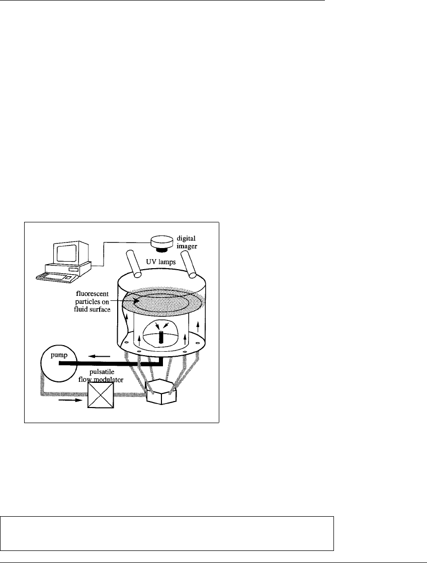
in Figure 6.16. The pump draws off some of the solution from the middle of the
Figure 6.16 Schematic view of the tank.
Sucrose solution is intermittently pumped out of the tank from the bottom and
returns through outlets in the bottom. Floating flourescent tracer particles (scum)
on the surface of the fluid are excited by ultraviolet lamps and photographed by a
digital camera.
Sommerer, J. 1994. Fractal tracer distributions in complicated surface flows: an application
of random maps to fluid dynamics. Physica D 76:85-98.
267
C HAOTIC ATTRACTORS
tank, and reinjects it at the bottom of the tank. There is a resulting mixing effect
on the fluid surface. After the pump is turned off, the fluid is allowed to come to
rest. The rest state of the fluid surface is by definition the result of one iteration
of the plane map.
In order to follow an individual trajectory, tiny tracer particles were dis-
tributed on the fluid surface. The particles were fluorescent plastic spheres, each
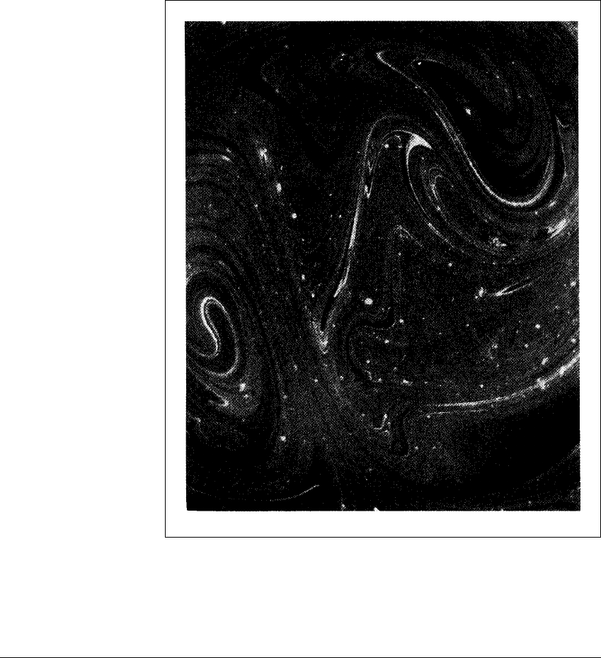
Figure 6.17 A 6-inch ⴛ 6-inch snapshot of the tracer distribution for the
pulsed flow.
Bright areas are due to a dense collection of the tracer material, which correspond
to a buildup of invariant measure. The distribution has a fractal appearance. This
exposure took several seconds.
268
L AB V ISIT 6
one being four one-thousandths of a millimeter in diameter. When ultraviolet
lamps were turned on, the tracer particles floating on the surface were illumi-
nated and photographed by the camera looking down on the surface. A typical
photograph is shown in Figure 6.17. The variations in the relative illumination
are caused by variations in the density of the tracer particles, which in turn ap-
proximate the natural measure of the attractor. Notice the pronounced fractal
structure caused by the mixing effects of the map.
This experiment should be modeled, strictly speaking, as a map with some
randomness. Due to the difficulty with exact control of the experimental condi-
tions, each time the pump is run, slightly different effects occur; the map applied
is not exactly the same each iteration, but an essentially random choice from a
family of quite similar maps. For such maps it is important to focus not so much
on individual trajectories but on collective, average behavior.
In order to estimate the Lyapunov exponents of this two-dimensional map,
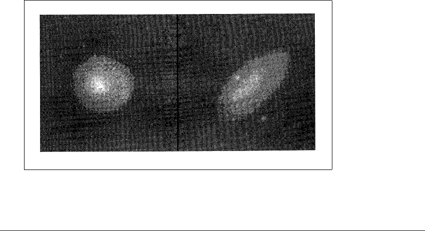
a different arrangement of tracer particles was used. A droplet of tracer was applied
to the surface with a pipette, forming a small disk as shown in Figure 6.18(a).
After the map is iterated once by running the pump as described, the disk becomes
an approximate ellipse as shown in Figure 6.18(b).
Determining the Lyapunov exponent from the definition would mean start-
ing with a tiny disk and observing the evolution of the ellipse for many iterations.
The stretching factor along the longest ellipse axis, when expressed on a per-step
basis, would give the Lyapunov number. However, this approach is impractical
Figure 6.18 Evolution of a disk under the map.
On the left is a circular tracer particle patch on the surface of the fluid. After a few
iterations of the map (pumping oscillations), the disk is transformed into an ellipse.
269
C HAOTIC ATTRACTORS
in this experiment. The ellipse cannot have an infinitesimal size, so it becomes
folded and distorted after just a few iterates.
This problem was solved by starting a new disk after each iteration. After
the first iteration, the ellipse of tracer particles is carefully removed by suction.
A new circular patch was placed at the point of removal, and a new iteration
commenced. Several dozen iterations were done in this way, and the ellipses
recorded. For each ellipse, the (geometric) average radius among all directions
of the ellipse was calculated. Then the geometric average of these radii over
all iterations was declared the dominant Lyapunov number. This is a reasonable
approximation for the Lyapunov number as long as the stretching directions of
the various ellipses are evenly distributed in two dimensions.
For each ellipse, the ratio of the ellipse area to the original disk area gives
an estimate for the Jacobian determinant of the map. Therefore the smaller of the
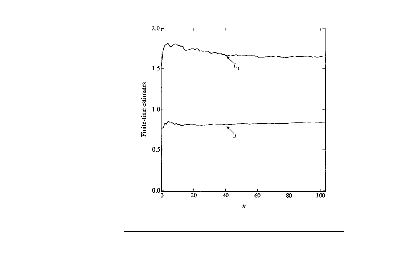
two Lyapunov numbers can also be found. The estimates for the larger Lyapunov
number 1.68 and the Jacobian determinant J ⫽ 0.83 are shown in Figure 6.19,
converging to their apparent limiting values after 100 iterations. Since we know
that the Lyapunov exponents satisfy
1
⫹
2
⫽ ln J, the Lyapunov exponents are
Figure 6.19 Convergence of the Lyapunov number estimate.
Experimental estimates of the largest Lyapunov number L
1
and area-contraction J.
270

L AB V ISIT 6
ln 1.68 ⫽ 0.52 and ⫺0.71. The Lyapunov dimension of the syrup attractor shown
in Figure 6.16 is therefore 1 ⫹ 0. 52 0.71 ⬇ 1.73.
This experiment was carried out and the results interpreted with consider-
ably more care than our description shows. In particular, great pains were taken to
correctly interpret the results in light of the random influences on the dynamics.
In addition, the experiment was repeated several times at different temperatures,
where the viscosity of the solution is different. At 38
◦
C, the syrup is runnier,
and the Lyapunov dimension is about 1.6. At 27
◦
C, the Lyapunov dimension is
estimated to be 1.9. Consult the original source for more details.
271

C HAPTER S EVEN
Differential Equations
I
NTHEFIRSTsix chapters, we modeled physical processes with maps. One of the
most important uses of maps in scientific applications is to assist in the study of
a differential equation model. We found in Chapter 2 that the time-T map of a
differential equation may capture the interesting dynamics of the process while
affording substantial simplification from the original differential equation.
A map describes the time evolution of a system by expressing its state as a
function of its previous state. Iterating the map corresponds to the system moving
through time in discrete updates. Instead of expressing the current state as a
function of the previous state, a differential equation expresses the rate of change
of the current state as a function of the current state.
273

D IFFERENTIAL E QUATIONS
A simple illustration of this type of dependence is Newton’s law of cooling,
which we discussed in Chapter 2. Consider the state x consisting of the difference
between the temperature of a warm object and the temperature of its surroundings.
The rate of change of this temperature difference is negatively proportional to
the temperature difference itself:
˙
x ⫽ ax, (7.1)
where a ⬍ 0. Here we have used the notation
˙
x to represent the derivative of
the function x. The solution of this equation is x(t) ⫽ x(0)e
at
, meaning that the
temperature difference x decays exponentially in time. This is a linear differential
equation, since the terms involving the state x and its derivatives are linear terms.
Another familiar example from Chapter 2, which yields a nonlinear differ-
ential equation, is that of the pendulum. The pendulum bob hangs from a pivot,
which constrains it to move along a circle, as shown in Figure 2.4 of Chapter 2.
The acceleration of the pendulum bob in the tangential direction is proportional
to the component of the gravitational downward force in the tangential direction,
which in turn depends on the current position of the pendulum. This relation of
the second derivative of the angular position with the angular position itself is
one of the most fundamental equations in science:
¨
x ⫽⫺sin x. (7.2)
The pendulum is an example of a nonlinear oscillator. Other nonlinear oscillators
that satisfy the same general type of differential equation include electric circuits,
feedback systems, and many models of biological activity.
Most physical laws that have been successful in the study of dynamically
changing quantities are expressed in the form of differential equations. The prime
example is Newton’s law of motion F ⫽ ma. The acceleration a is the second
derivative of the position of the object being acted upon by the force F. Newton
and Leibniz developed the calculus in the seventeenth century to express the fact
that a relationship between x and its derivatives
˙
x,
¨
x and so on, can determine
the motion in the past and future, given a specified present (initial condition).
Since then, calculus and differential equations have become essential tools in the
sciences and engineering.
Ordinary differential equations are differential equations whose solutions
are functions of one independent variable, which we usually denote by t.The
variable t often stands for time, and the solution we are looking for, x(t), usually
stands for some physical quantity that changes with time. Therefore we consider
x as a dependent variable. Ordinary differential equations come in two types:
274

7.1 ONE-DIMENSIONAL L INEAR D IFFERENTIAL E QUATIONS
• Autonomous, for example
˙
x ⫽ ax, (7.3)
in which the time variable t does not explicitly appear, and
• Nonautonomous, as in the forced damped pendulum equation
¨
x ⫽⫺c
˙
x ⫺ sin x ⫹
sin t, (7.4)
for which t appears explicitly in the differential equation.
Autonomous differential equations are the ones that directly capture the spirit of
a deterministic dynamical system, in which the law for future states is written only
in terms of the present state x. However, the distinction is somewhat artificial: Any
nonautonomous equation can be written as an autonomous system by defining a
new dependent variable y equal to t; then for example we could write (7.4) as
¨
x ⫽⫺c
˙
x ⫺ sin x ⫹
sin y
˙
y ⫽ 1. (7.5)
The system of equations (7.5) is autonomous because t does not appear on the
right-hand side. In effect, t has been turned into one of the dependent variables
by renaming it y. Because autonomous equations are the more general form, we
will restrict our attention to them in this chapter.
The order of an equation is the highest derivative that occurs in the equa-
tion. We will begin by discussing first-order equations, in which only first deriva-
tives of the dependent variable occur. The equations may be linear or nonlinear,
and there may be one or more dependent variables. We will discuss several cases,
in order of increasing complexity.
7.1 ONE-DIMENSIONAL LINEAR
DIFFERENTIAL EQUATIONS
First, let us explain the title of this section. The dimension refers to the number
of dependent variables in the equation. In this section, there is one (the variable
x), which is a function of the independent variable t. The differential equation
will express
˙
x, the instantaneous rate of change of x with respect to t,intermsof
the current state x of the system. If the expression for
˙
x is linear in x, we say that
it is a linear differential equation.
275
D IFFERENTIAL E QUATIONS
Let
˙
x ⬅
dx
dt
⫽ ax, (7.6)
where x is a scalar function of t, a is a real constant, and
˙
xdenotes the instantaneous
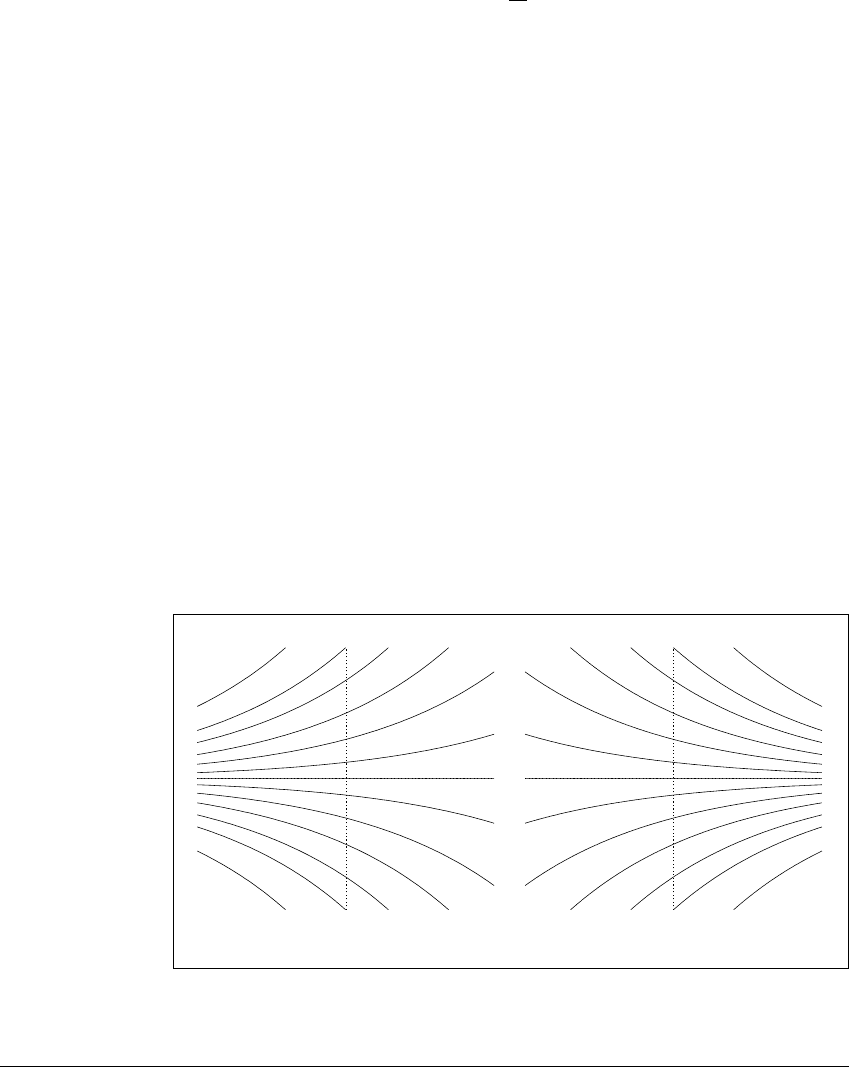
rate of change with respect to time. For a ⬎ 0, (7.6) is a simple model of population
growth when the population is small. The rate dx dt at which the population grows
is proportional to the size x of the population. Solutions of (7.6) with a ⬎ 0are
shown in Figure 7.1(a). (Compare these with the population model x
n⫹1
⫽ ax
n
in Chapter 1. In that case, the size of the new population is proportional to the
previous population. These are different models.)
The differential equation (7.6) has infinitely many solutions, each of form
x(t) ⫽ ce
at
, for a constant real number c. By substituting t ⫽ 0, it follows that
x(0) ⫽ c. The number x
0
⫽ x(0) is called the initial value of the function x.A
problem is usually stated in the form of an initial value problem, which consists
of a differential equation together with enough initial values (one, in this case)
to specify a single solution. Using this terminology, we say that the solution of
the initial value problem
˙
x ⫽ ax
x(0) ⫽ x
0
(7.7)
is
x(t) ⫽ x
0
e
at
. (7.8)
x
t
x
t
x
t
x
t
x
t
(a) (b)
Figure 7.1 The family of solutions of ˙
x
ⴝ
ax
.
(a) a ⬎ 0: exponential growth (b) a ⬍ 0: exponential decay.
276